Week 5 - Genetic Algorithm
Genetic Algorithm
AIM : To study about Genetic Algorithm and to calculate the global maxima of stalagmite function using Genetic Algorithm in MATLAB.
OBJECTIVE :
- To write a code in Matlab to optimise the stalagmite function and find the global maxima of the function and plot graphs based on the studies done for Genetic Algorithm.
- Genetic Algorithm and Stalagmite function.
Description:
The genetic algorithm is inspired by the process that drives biological evaluation.
The process of evaluation starts with the selection of fittest individuals from a population.
This process keeps on iterating and at the end, a generation with the fittest individuals will be found.
And this is the main working principle for the algorithm because at each step, the genetic algorithm selects randomly from the current populations to be parents and uses them to produce the children for the next generation.Over successive generations, the population evolves towards an optimal solution. The genetic algorithm can be applied to solve a variety of optimization problems that are not well suited for standard optiization algorith, including problems i which the objective function is discontinuous, non-differentiable, or highly nonlinear.
Optimization:
- Optimization is the process of selection from the set of values for the imposed targets and the constraints.
- process handling mayny parameters ,where its integrated with each other and afffects one another in all aspects.
- It is been very dificult to manage and select the appropriate range of values for the defined targets and constraints.
- To make this process ease,optimization technique helps us to find a way to get the best out of it.
Stalagmite function:
- A stalagmite is an upward-growing mound of mineral deposits that have precipitated from water dripping onto the floor of a cave. Most stalagmites have rounded or flattened tips.
- A stalagmite function generally refers to the function with which we are generating values over a stalagmite kind of surface for finding out the local and global maxima and minima of that particular given function.
Genetic Algorithm –
The genetic algorithm uses three main types of rules at each step to create the next generation from the current population and the basic steps in creating a genetic algorithm are
- Selection rules select the individuals called parents, that contribute to the population at the next generation.
- Crossover rules combine two parents to form children for the next generation.
- Mutation rules apply random changes to individual parents to form children.
- The algorithm creates a random initial population at beginning.
- Then to create new population, the algorithm scores each member of the current population by computing its fitness value and converts them into a more usable range of values.
- Then based on these new values the algorithm selects members, called as parents.
- Then the algorithm produces children from the parents. Children are produced either by making random changes to a single parent which is mutation or by combining the vector entries of a pair of parents which is crossover.
- In this way the algorithm replaces the current population with the children to form the next generation.
- The algorithm stops when it reaches any one of the specified factors factors such as time limit, fitness limit, generations, function tolerance, constraint tolerance, etc.
GA Syntax:
x=ga(fun,nvars,A,b,Aeq,beq,lb,ub,nonlcon,options)
Where fun= objective function.
nvar= number of variables.(specified as positive integers)
A,b=linear inequality constraints (A=Real matrix ,b=real vector)
Aeq,beq= Linear equality constraints (A=Real matrix ,b=real vector)
Lb,Ub= Lower bounds and upper bounds
nonlcon= Nonlinear constraints
options= Optimization options
Algorithm Working Sequence :-
Algorithm then creates a sequence of new populations. At each step, the algorithm uses the individuals in the current generation to create the next population. To create the new population, it uses the fitness function which is the function you want to optimize.For standard optimization algorithms, this is known as the objective function.The toolbox software tries to find the minimum of the fitness function.
The algorithm performs the following steps-
- The algorithm begins by creating a random initialpopulations
- Then it scales the raw fitness scores to convert them into a more usable range of values. These scaled values are called expectation values.
- Then it selects members,called parents, based on their expectations.
- Along the individual that have high fitness value, some of the individuals i the current population that have lower fitness are chosen as elite. These elite individuals are passed to the next populations. Also it produces children by making random changes to a single parents-mutation-or by combining the vector entries of a pair of parents-crossover.
- It then replaces the current population with the children to form the next generation.
- Then it scores each member of the current population by computing it's fitness value. These values are called the raw fitness scores
- Then the algorithm stops when one of the stopping criteria is met
Input Function :-
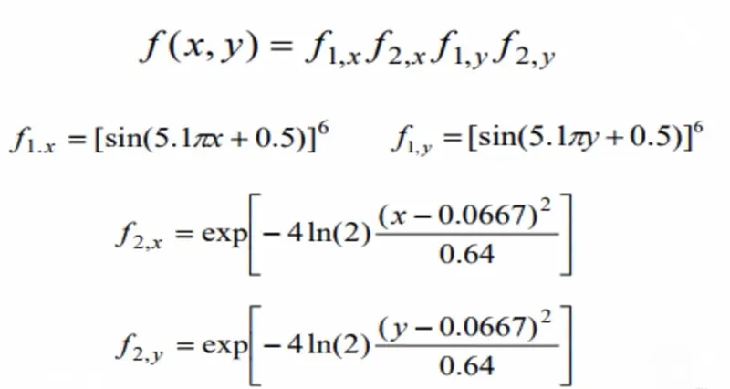
The above equations are used in the stalagmite function to plot the graph in the main functions-
function [f] = stalagmite(input_value)
f = -(f1x*f1y*f2x*f2y);
end
While using the function at the end as we are using the -ve sign so that the plot will be reversed as we have to find the maxima of the given function using ga.
3.PROGRAM DESCRIPTION:
1.In this program we will first give x an y array by using linspace command here it is like
x=linspace(0,0.6,150);
- In case-1: as shown in the code we are going to run the code for 50 iterations thats why we have taken ,
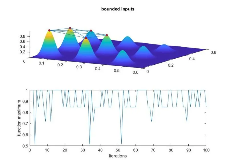
- In case -2 :We are going to use the same thing that we did earlier but here we will be providing some boundary condition to the ga i.e. we have provided boundary conditions to ga function .
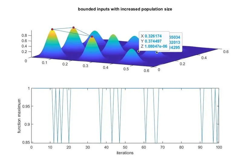
- In Case-3 :In this study using the ‘optimoptions’ command to increase the size of population and the benefit of that will be it will be working on the large set of numbers and which will be led to increase the possibilities of finding the better fitness of the function.
function [f]=stalagmite(input_vector)
x=input_vector(1);
y=input_vector(2);
f1x=(sin((5.1*pi*x)+0.5))^6;
f1y=(sin((5.1*pi*y)+0.5))^6;
f2x=exp(-4*log(2)*(((x-0.0667)^2)/0.64));
f2y=exp(-4*log(2)*(((y-0.0667)^2)/0.64));
f=-(f1x*f1y*f2x*f2y);
end
Main code
clear all
close all
clc

x=linspace(0,0.6,150);
y=linspace(0,0.6,150);

% creating a two dimensional mesh
[xx yy]=meshgrid(x,y);

%evaluating the stalagmite function
for i=1:length(xx)
    for j=1:length(yy);
        input_vector(1)=xx(i,j);
        input_vector(2)=yy(i,j);
        f(i,j)=stalagmite(input_vector);
    end
end

% GA runs for 100 iterations
num_cases=100
% Study Time count start
tic

% Study-1 statistical behaviour
for i=1:num_cases
    % GA function is used to run the stalagmite data and give the optimal solutions.
    [inputs,fopt(i)]=ga(@stalagmite,2);
    xopt(i)=inputs(1);
    yopt(i)=inputs(2);
    %Ga gives us Minima value.Inverse f_opt is taken for Maxima value
    optf(i)=-fopt(i)
end

% Study Time count end
study1_time = toc


figure(1)
subplot(2,1,1)
hold on
%Generation of stalagmite function.
surfc(xx,yy,-f)
% To bring visually smooth curve surface without mesh lines
shading interp
%plotting the optimum values with a red dot marker along the stalagmite 3D curves
plot3(xopt,yopt,optf,'marker','o','MarkerSize',5,'MarkerFaceColor','r')
title('unbounded inputs')
subplot(2,1,2)
%plot of opt_f for every iterations
plot(optf)
xlabel('iterations')
ylabel('function maximum')

% Study Time count start
    tic


    % Study 2-statistical behaviour with upper and lower bounds
    for i=1:num_cases
        % GA function is used to run the stalagmite data and give the optimal solutions.
        [inputs,fopt(i)]=ga(@stalagmite,2,[],[],[],[],[0;0],[1,1]);
        xopt(i)=inputs(1);
        yopt(i)=inputs(2);
        %Ga gives us Minima value.Inverse f_opt is taken for Maxima value
        optf(i)=-fopt(i)
    end

    % Study Time count end
    study2_time=toc

    figure(2)
    subplot(2,1,1)
    hold on
    %Generation of stalagmite function.
    surfc(xx,yy,-f)
    % To bring visually smooth curve surface without mesh lines
    shading interp
    plot3(xopt,yopt,optf,'marker','o','MarkerSize',5,'MarkerFaceColor','r')
    title('bounded inputs')
    subplot(2,1,2)
    %plot of opt_f for every iterations
    plot(optf)
    xlabel('iterations')
    ylabel('function maximum')

    % Study Time count start
    tic

    % Study-3 increasing GA iterations
     % optimoptions is used to increase population size
options=optimoptions('ga');
options=optimoptions(options,'populationsize',  170);

 tic

    for i=1:num_cases
        % GA function is used to run the stalagmite data and give the optimal solutions.
        [inputs,fopt(i)]=ga(@stalagmite,2,[],[],[],[],[0;0],[1,1],[],[],options);
        xopt(i)=inputs(1);
        yopt(i)=inputs(2);
        %Ga gives us Minima value.Inverse f_opt is taken for Maxima value
        optf(i)=-fopt(i)
    end

    % Study Time count end
    study3_time=toc

    figure(3)
    subplot(2,1,1)
    hold on
    %Generation of stalagmite function.
    surfc(xx,yy,-f)
    % To bring visually smooth curve surface without mesh lines
    shading interp
    plot3(xopt,yopt,optf,'marker','o','MarkerSize',5,'MarkerFaceColor','r')
    title('bounded inputs with increased population size')
    subplot(2,1,2)
    %plot of opt_f for every iterations
    plot(optf)
    xlabel('iterations')
    ylabel('function maximum')
Error
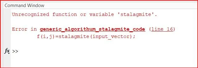
- Error resolved by calling the right function name as saved in the folder
Output
Study time
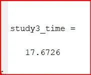
Result of Statistical Study
Study 1 : UNBOUNDED
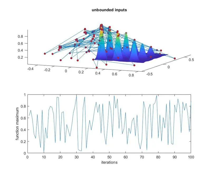
Study 2 : BOUNDED
Study 3 : BOUNDED INPUTS WITH INCREASED POPULATION SIZE
REFERENCES: