Week 5 - Genetic Algorithm
GENETIC ALGORITHM
AIM:-
- Write a code in MATLAB to optimise the stalagmite function and find the global maxima of the function.
- Clearly explain the concept of genetic algorithm in your own words and also explain the syntax for ga in MATLAB in your report.
- Make sure that your code gives the same output, even if it is made to run several times.
- Plot graphs for all 3 studies and for F maximum vs no. of iterations. Title and axes label are a must, legends could be shown if necessary.
EXPLAIN THEORY-
The genetic algorithm is a method for solving both constrained and unconstrained optimization problems that is based on natural selection, the process that drives biological evolution such as mutation, crossover, and selection. Optimization is a procedure that is executed iteratively by comparing various solutions until an optimum or a satisfactory solution is found. Optimization refers to finding the values of inputs in such a way that we get the best output values. That is why genetic algorithm is one of the optimization processes.
There are five important features of Genetic Algorithm.
- To set of individuals involved in the process is called as population. Each individual is a solution to the problem you want to solve.
- The fitness function which determines how fit an individual is to compete with others.
- The selection is the phase of selecting the more fittest individuals. Individuals with high fitness value have more chance to get selected.
- The crossover is the most significant phase in a genetic algorithm, for each pair of parents to be mated, a crossover point is chosen at random from within the genes.
- The mutation occurs to maintain diversity within the population and prevent premature convergence.
STALAGMITE FUNCTION :-
The stalagmite function model will help us to generate local maxima and minima. A stalagmite is the type of rock formation that rise from the floor of the cave due to the accumulation of materials deposited on the floor from ceiling drippings. Stalagmite may be composed of lava, minerals, sands etc.
CODE WITH LINE BY LINE EXPLANATION:-
FUNCTION CODE:-
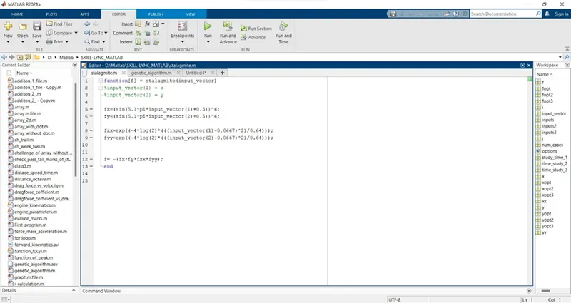
function[f] = stalagmite(input_vector)
%input_vector(1) = x
%input_vector(2) = y
fx=(sin(5.1*pi*input_vector(1)+0.5))^6;
fy=(sin(5.1*pi*input_vector(2)+0.5))^6;
fxx=exp((-4*log(2)*(((input_vector(1)-0.0667)^2)/0.64)));
fyy=exp((-4*log(2)*(((input_vector(2)-0.0667)^2)/0.64)));
f= -(fx*fy*fxx*fyy);
end
EXPLANATION-
First we created a function from equation f input vector 1&2. And then we write the code for formula to find the value of f. generating algorithm will only find lowest value using stalagmite command function. To find the global maxima I have use (-) sign in final formula. And save this file where main code is save with same function name.
MAIN CODE WITH LINE BY LINE EXPLANATION:-
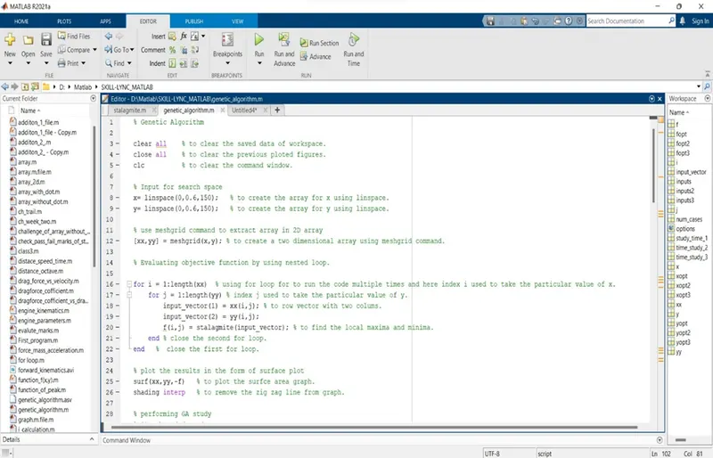
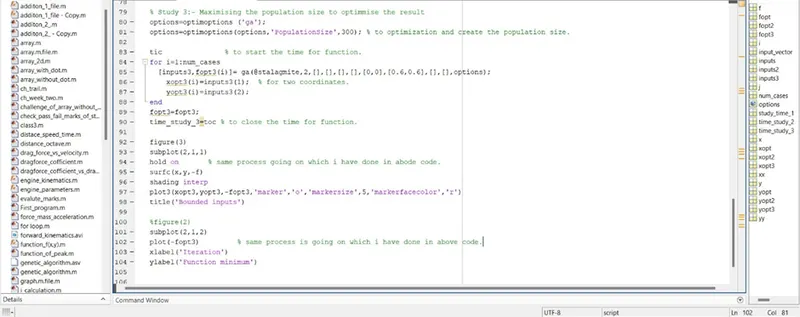
% Genetic Algorithm
clear all % to clear the saved data of workspace.
close all % to clear the previous ploted figures.
clc % to clear the command window.
% Input for search space
x= linspace(0,0.6,150); % to create the array for x using linspace.
y= linspace(0,0.6,150); % to create the array for y using linspace.
% use meshgrid command to extract array in 2D array
[xx,yy] = meshgrid(x,y); % to create a two dimensional array using meshgrid command.
% Evaluating objective function by using nested loop.
for i = 1:length(xx) % using for loop for to run the code multiple times and here index i used to take the particular value of x.
for j = 1:length(yy) % index j used to take the particular value of y.
input_vector(1) = xx(i,j); % to row vector with two colums.
input_vector(2) = yy(i,j);
f(i,j) = stalagmite(input_vector); % to find the local maxima and minima.
end % close the second for loop.
end % close the first for loop.
% plot the results in the form of surface plot
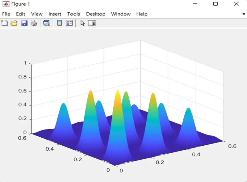
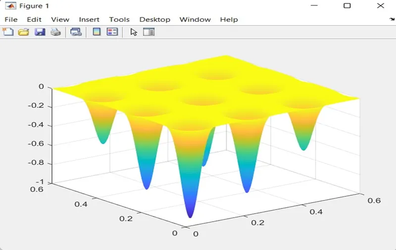
surf(xx,yy,-f) % to plot the surfce area graph.
shading interp % to remove the zig zag line from graph.
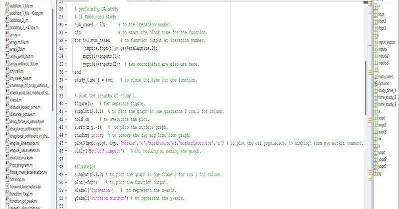
% performing GA study
% 1) Unbounded study
num_cases = 50; % to the iteration number.
tic % to start the clock time for the function.
for i=1:num_cases % to fucntion output at iteration number.
[inputs,fopt(i)]= ga(@stalagmite,2);
xopt(i)=inputs(1);
yopt(i)=inputs(2); % two coordinates are also use here.
end
study_time_1 = toc; % to close the time for the function.
% plot the results of study 1
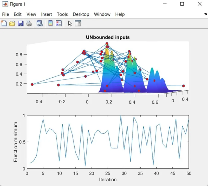
figure(1) % for separate figure.
subplot(2,1,1) % to plot the graph in one quadrants 2 row,1 for column.
hold on % to overwrite the plot.
surfc(x,y,-f) % to plto the surface graph.
shading interp % to remove the zig zag line from graph.
plot3(xopt,yopt,-fopt,'marker','o','markersize',5,'markerfacecolor','r') % to plot the all population, to highligh them use marker command.
title('Bounded iinputs') % for heading or naming the graph.
%figure(2)
subplot(2,1,2) % to plot the graph in one frame 2 for row 1 for column.
plot(-fopt) % to plot the function output.
xlabel('Iteration') % to represent the x-axis.
ylabel('Function minimum') % to represent the y-axis.
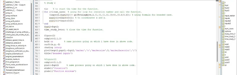
% Study 2
tic % to start the time for the function.
for i=1:num_cases % using for loop for iteration number and call the function.
[inputs2,fopt2(i)]= ga(@stalagmite,2,[],[],[],[],[0;0],[0.6;0.6]); % using formula for bounded case.
xopt2(i)=inputs2(1); % to coordinates x and y.
yopt2(i)=inputs2(2);
end
fopt2=fopt2;
time_study_2=toc; % close the time for fucntion.
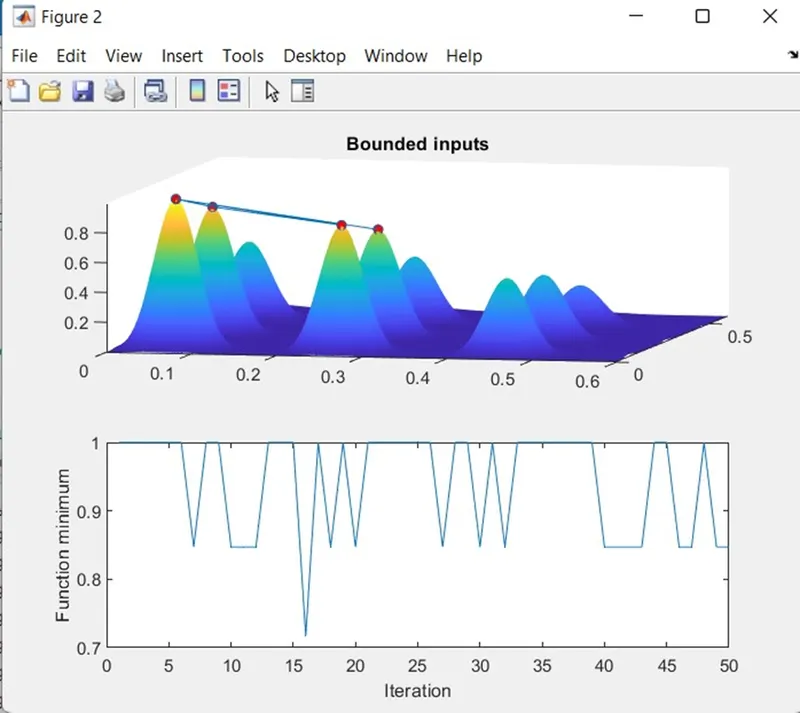
figure(2)
subplot(2,1,1)
hold on % same process going on which i have done in above code.
surfc(x,y,-f)
shading interp
plot3(xopt2,yopt2,-fopt2,'marker','o','markersize',5,'markerfacecolor','r')
title('Bounded inputs')
%figure(2)
subplot(2,1,2)
plot(-fopt2) % same process going on which i have done in above code.
xlabel('Iteration')
ylabel('Function minimum')
% Study 3:- Maximising the population size to optimmise the result
options=optimoptions ('ga');
options=optimoptions(options,'PopulationSize',300); % to optimization and create the population size.
tic % to start the time for function.
for i=1:num_cases
[inputs3,fopt3(i)]= ga(@stalagmite,2,[],[],[],[],[0,0],[0.6,0.6],[],[],options);
xopt3(i)=inputs3(1); % for two coordinates.
yopt3(i)=inputs3(2);
end
fopt3=fopt3;
time_study_3=toc % to close the time for function.
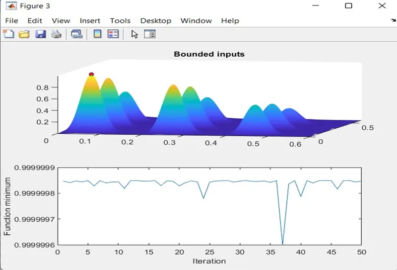
figure(3)
subplot(2,1,1)
hold on % same process going on which i have done in abode code.
surfc(x,y,-f)
shading interp
plot3(xopt3,yopt3,-fopt3,'marker','o','markersize',5,'markerfacecolor','r')
title('Bounded inputs')
%figure(2)
subplot(2,1,2)
plot(-fopt3) % same process is going on which i have done in above code.
xlabel('Iteration')
ylabel('Function minimum')
EXPLANATION-
- Clear all – clear all the data stored in the workspace.
- Close all – clear all the previous plot and figure.
- Clc – clear the command window
- First give the input for x and y using linspace command. Then use meshgrid command for two dimensional array represented by xx and yy.
- After that start the for loop for the length of the xx and yy, the input is a row vector with two column which we are assigning using input vector 1&2.
- For call the function,Using stalagmite function for defined the local maxima and minima.
- Then plot the graph use surf command and shading interp to remove the zig zag line from graph.
- Then performing ga study.
- For that use num_cases for iteration number.
- For unbounded study start for loop and call the function and plot the graph with all xlabel, ylabel and legend.
- After that same process going on for next two study of genetic algorithm.
- And plot the graph.
- After that save the file in same path with function code.
- After that run the code and we will get the result.
RESULT-
STALAGMITE FUNCTION-
UNBOUNDED STUDY-
BOUNDED STUDY
BOUNDED STUDY WITH MODIFIED POPULATION SIZE-
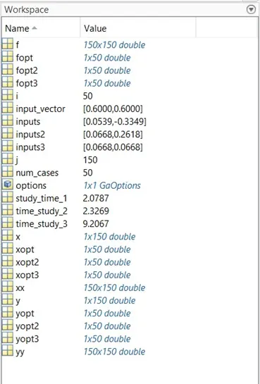
RESULT IN WORKSPACE-
ERROR AND SOLUTION-
ERROR 1-

SOLUTION 1-

To upward graph we have to use the (-f)sign.
ERROR 2-
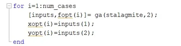
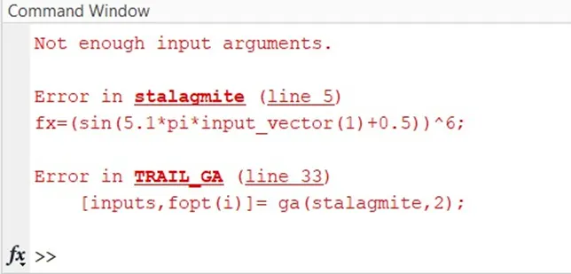
SOLUTION 2-
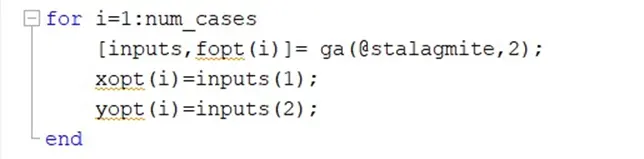
To fix that error I had use the as the rate(@)symbol.
ERROR 3-

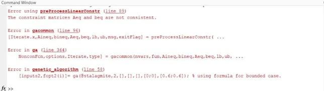
SOLUTION 3-

To solve this problem I have used the one extra open bracket[].