Week 5 - Genetic Algorithm

Aim:

The aim of the report is to explain genetic algorithms and their application in optimizing the stalagmite function. It will detail the syntax of the ga function in MATLAB and provide code to find the global maximum of the function. The report will present results from three case studies, analyzing the behavior of the genetic algorithm under different conditions. Graphs will illustrate the surface plot of the function and the convergence of the maximum over iterations. Overall, the report aims to demonstrate the effectiveness of genetic algorithms for optimization tasks.

Objective:

• Explain the concept of genetic algorithms and their application in optimization problems.
• Introduce the stalagmite function and its mathematical formulation.
• Present the syntax of the ga function in MATLAB for optimization.
• Provide MATLAB code to optimize the stalagmite function and find its global maximum.
• Conduct three case studies to analyze the behavior of the genetic algorithm under different conditions.
• Illustrate results with graphs showing the surface plot of the function and the convergence of the maximum over iterations.

Problem Statement:

To optimize the stalagmite function and find its global maximum using genetic algorithms in MATLAB, while exploring the behavior of the algorithm under various conditions and analyzing its convergence characteristics.

Stalagmites

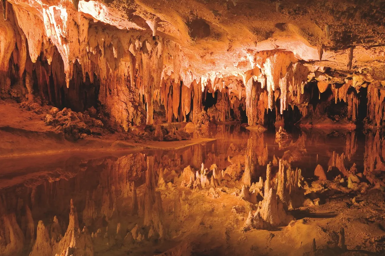
Stalagmites are mineral formations that rise from the floor of caves due to the accumulation of mineral-rich water dripping from the ceiling. They typically form over long periods of time as dissolved minerals precipitate out of the water and build up layer by layer. Stalagmites often exhibit unique shapes and patterns, influenced by factors such as the mineral composition of the water, the rate of dripping, and the airflow within the cave.

In the context of optimization algorithms, the stalagmite function is a mathematical representation inspired by the natural formation of stalagmites. It typically involves multiple variables and complex equations, with the objective of finding the global maximum or minimum of the function. The stalagmite function serves as a challenging optimization problem that can be used to test and compare the performance of different optimization algorithms, including genetic algorithms.

General Algorithm (GA)

Genetic algorithm (GA) was first used by John Holland Adaptation in Natural and Artificial Systems of 1975. Genetic Algorithms are a family of computational models inspired by evolution. Genetic algorithms are often viewed as function optimizers although the range of problems to which genetic algorithms have been applied is quite broad.

The genetic algorithm is a method for solving both constrained and unconstrained optimization problems that is based on natural selection, the process that drives biological evolution. The genetic algorithm repeatedly modifies a population of individual solutions. At each step, the genetic algorithm selects individuals from the current population to be parents and uses them to produce the children for the next generation. Over successive generations, the population "evolves" toward an optimal solution. You can apply the genetic algorithm to solve a variety of optimization problems that are not well suited for standard optimization algorithms, including problems in which the objective function is discontinuous, nondifferentiable, stochastic, or highly nonlinear. The genetic algorithm can address problems of mixed integer programming, where some components are restricted to be integer-valued.

A procedural implementation of a genetic algorithm shown in figure 1:

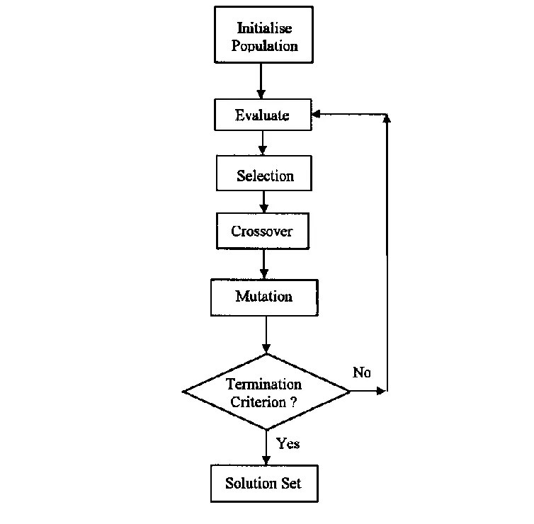
Fig.1. Basic Architecture of Genetic Algorithm

Here are the different phases of a genetic algorithm:

1. Initialization: The algorithm starts by creating a random population of individuals. Each individual represents a possible solution to the problem. In this context, an individual is called a chromosome, and it consists of genes, which are the parameters that define the solution. For example, if you're trying to optimize the design of a bridge, a chromosome might represent the length, width, and type of material used for the bridge.

2. Fitness Evaluation: Each individual in the population is evaluated using a fitness function. The fitness function determines how well an individual solution solves the problem. Individuals with higher fitness scores are considered more likely to survive and reproduce.

3. Selection: Based on their fitness scores, a selection process is used to choose which individuals will be parents and reproduce. There are different selection methods, but common ones include roulette wheel selection and tournament selection. Roulette wheel selection assigns a probability of selection to each individual based on its fitness score. Individuals with higher fitness scores have a larger slice of the pie and are therefore more likely to be selected. Tournament selection involves randomly selecting a small group of individuals and choosing the fittest one from that group to be a parent.

4. Reproduction: Once the parents are selected, they reproduce to create offspring. This involves two main mechanisms: crossover and mutation. Crossover involves combining the genetic material of two parents to create new offspring. Mutation involves randomly changing some of the genes in an offspring. Crossover helps to explore new regions of the search space, while mutation helps to prevent the population from getting stuck in a local optimum.

   • Crossover: This simulates mating, where genetic material from two parents is combined to create new offspring. By exchanging genes, crossover helps explore different combinations of existing solutions.

   • Mutation: This mimics random biological mutations. It introduces small changes to the offspring's genes with a low probability. Mutation helps maintain diversity in the population and prevents getting stuck in local optima (suboptimal solutions).

5. Termination: The algorithm continues to iterate through these steps (evaluation, selection, reproduction) until a termination criterion is met. Common termination criteria include reaching a maximum number of generations, finding a solution with a sufficiently good fitness score, or the population converging on a small set of solutions.

Genetic algorithms are a powerful tool for solving a wide range of optimization problems. They are particularly well-suited for problems where the search space is large and complex, and where there is no known formula for finding the optimal solution.

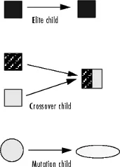
The genetic algorithm uses three main types of rules at each step to create the next generation from the current population:

Syntax for 'ga' in Matlab:

The ga function syntax is as follows:

[x, fval] = ga(fun, nvars, A, b, Aeq, beq, lb, ub, nonlcon, options)

• fun: This is a function handle that points to the objective function you want to minimize. It should take a vector of decision variables as input and return a scalar value representing the objective function value.

• nvars: This is an integer specifying the number of decision variables in your optimization problem.

• A, b: These are optional arguments that define linear inequality constraints. A is a matrix where each row represents a constraint, and b is a vector containing the right-hand sides of the constraints. The constraints are defined as A * x <= b.

• Aeq, beq: These are optional arguments that define linear equality constraints. Similar to A and b, Aeq is a matrix for constraints, and beq is a vector for the right-hand sides. The constraints are defined as Aeq * x == beq.

• lb, ub: These are optional arguments that define lower and upper bounds for the decision variables. lb is a vector containing the lower bounds, and ub is a vector containing the upper bounds.

• nonlcon: This is an optional argument that allows you to specify non-linear constraints using a function handle. This function should take a vector of decision variables as input and return a vector of constraint values.

• options: This is an optional argument that allows you to specify various options for the genetic algorithm, such as population size, selection method, crossover rate, mutation rate, and termination criteria. You can use the optimoptions function to create a structure containing these options.

Here are some additional points to note:

• The ga function returns two outputs:
  • x: This is a vector containing the solution (optimal decision variables) found by the genetic algorithm.
  • fval: This is the scalar value of the objective function evaluated at the solution x.
• By default, ga minimizes the objective function. If you want to maximize the function, you can negate the function value inside your fun function handle.
• The ga function is a part of the Global Optimization Toolbox in MATLAB. You may need to install this toolbox to use the function.

Matlab Program:

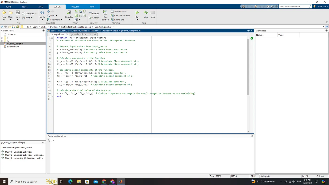
Function Block File (Stalagmite)

function [f] = stalagmite(input_vector)
% Function to calculate the value of the "stalagmite" function

% Extract input values from input_vector
x = input_vector(1); % Extract x value from input vector
y = input_vector(2); % Extract y value from input vector

% Calculate components of the function
f1_x = (sin(5.1*pi*x + 0.5)).^6; % Calculate first component of x
f1_y = (sin(5.1*pi*y + 0.5)).^6; % Calculate first component of y

% Calculate second components of the function
t1 = (((x - 0.0667).^2)/(0.64)); % Calculate term for x
f2_x = exp(-4.*log(2)*t1); % Calculate second component of x

t2 = (((y - 0.0667).^2)/(0.64)); % Calculate term for y
f2_y = exp(-4.*log(2)*t2); % Calculate second component of y

% Calculate the final value of the function
f = -(f1_x.*f2_x.*f1_y.*f2_y); % Combine components and negate the result (negative because we are maximizing)
end

Explanation:

Input Extraction

x = input_vector(1);
y = input_vector(2);

Here, the code extracts the values of x and y from the input_vector argument. input_vector is assumed to be a 2-element vector containing the values of x and y.

Components Calculation

f1_x = (sin(5.1*pi*x + 0.5)).^6;
f1_y = (sin(5.1*pi*y + 0.5)).^6;

These lines calculate the first components of the function. Each component involves taking the sine of a specific expression (5.1*pi*x + 0.5 for x and 5.1*pi*y + 0.5 for y) and then raising the result to the power of 6.

Second Components Calculation

t1 = (((x - 0.0667).^2)/(0.64));
f2_x = exp(-4.*log(2)*t1);

t2 = (((y - 0.0667).^2)/(0.64));
f2_y = exp(-4.*log(2)*t2);

These lines calculate the second components of the function. Each component involves calculating a term (t1 for x and t2 for y) and then exponentiating it. The terms t1 and t2 are calculated as the square of the difference between the input value and 0.0667, divided by 0.64.

Final Function Calculation

f = -(f1_x.*f2_x.*f1_y.*f2_y);

Finally, these lines combine all the components calculated above to compute the final value of the function. The components are multiplied together, and the negative sign is applied to the result. This indicates that the function is being maximized rather than minimized.

Overall Function Purpose

The purpose of this code is to define a MATLAB function named stalagmite that calculates the value of a specific mathematical function. The function takes a 2-element input vector [x, y] and returns a scalar value f based on the calculations described above. The function appears to involve sinusoidal and exponential terms, and it's designed for optimization, as indicated by the negation of the final result.

Main Code File (Genetic Algorithm Study)

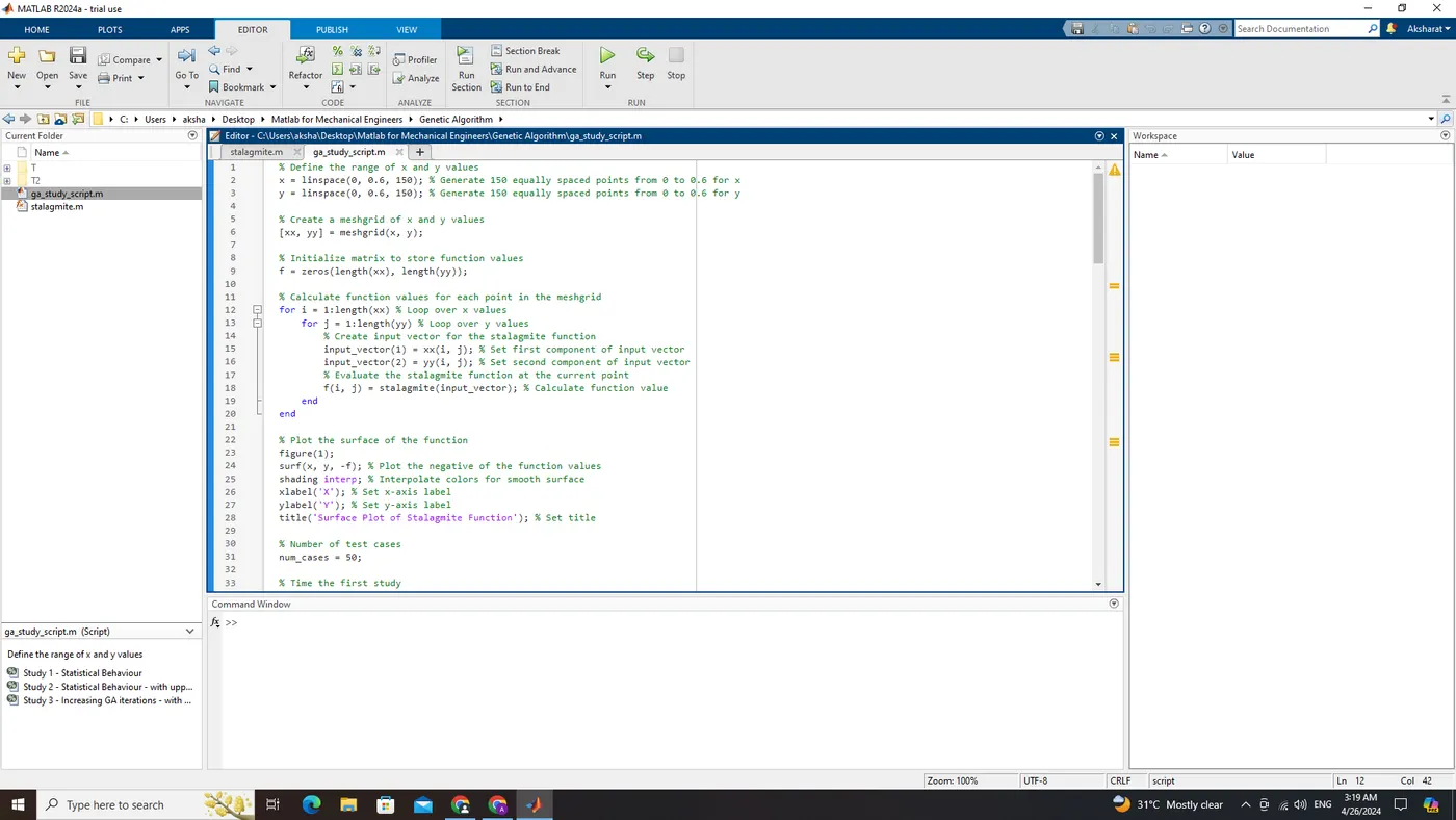
% Define the range of x and y values
x = linspace(0, 0.6, 150); % Generate 150 equally spaced points from 0 to 0.6 for x
y = linspace(0, 0.6, 150); % Generate 150 equally spaced points from 0 to 0.6 for y

% Create a meshgrid of x and y values
[xx, yy] = meshgrid(x, y);

% Initialize matrix to store function values
f = zeros(length(xx), length(yy));

% Calculate function values for each point in the meshgrid
for i = 1:length(xx) % Loop over x values
    for j = 1:length(yy) % Loop over y values
        % Create input vector for the stalagmite function
        input_vector(1) = xx(i, j); % Set first component of input vector
        input_vector(2) = yy(i, j); % Set second component of input vector
        % Evaluate the stalagmite function at the current point
        f(i, j) = stalagmite(input_vector); % Calculate function value
    end
end

% Plot the surface of the function
figure(1);
surf(x, y, -f); % Plot the negative of the function values
shading interp; % Interpolate colors for smooth surface
xlabel('X'); % Set x-axis label
ylabel('Y'); % Set y-axis label
title('Surface Plot of Stalagmite Function'); % Set title

% Number of test cases
num_cases = 50;

% Time the first study
tic;

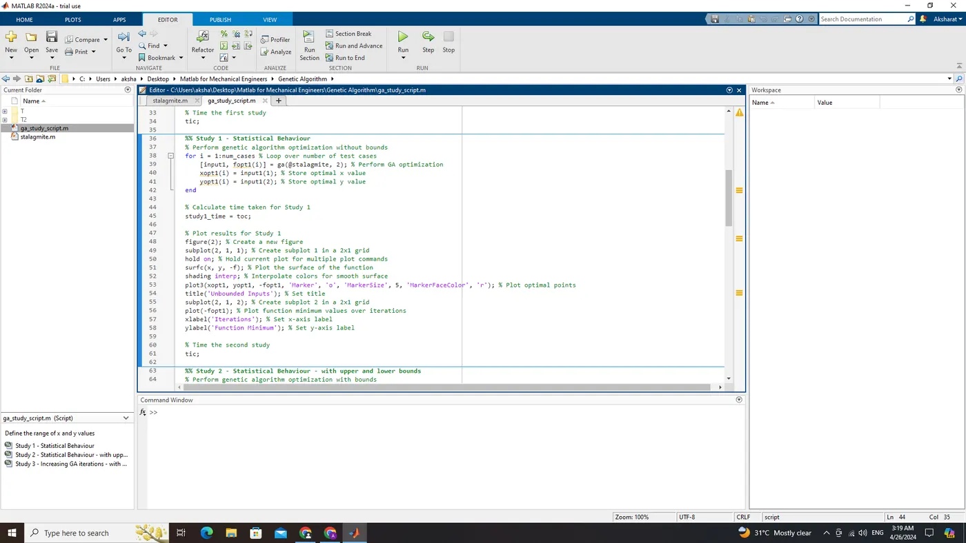
%% Study 1 - Statistical Behaviour
% Perform genetic algorithm optimization without bounds
for i = 1:num_cases % Loop over number of test cases
    [input1, fopt1(i)] = ga(@stalagmite, 2); % Perform GA optimization
    xopt1(i) = input1(1); % Store optimal x value
    yopt1(i) = input1(2); % Store optimal y value
end

% Calculate time taken for Study 1
study1_time = toc;

% Plot results for Study 1
figure(2); % Create a new figure
subplot(2, 1, 1); % Create subplot 1 in a 2x1 grid
hold on; % Hold current plot for multiple plot commands
surfc(x, y, -f); % Plot the surface of the function
shading interp; % Interpolate colors for smooth surface
plot3(xopt1, yopt1, -fopt1, 'Marker', 'o', 'MarkerSize', 5, 'MarkerFaceColor', 'r'); % Plot optimal points
title('Unbounded Inputs'); % Set title
subplot(2, 1, 2); % Create subplot 2 in a 2x1 grid
plot(-fopt1); % Plot function minimum values over iterations
xlabel('Iterations'); % Set x-axis label
ylabel('Function Minimum'); % Set y-axis label

% Time the second study
tic;

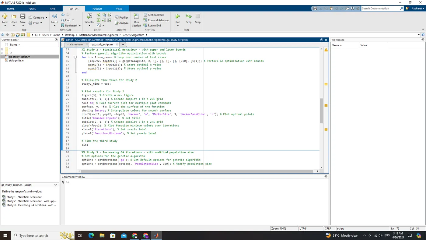
%% Study 2 - Statistical Behaviour - with upper and lower bounds
% Perform genetic algorithm optimization with bounds
for i = 1:num_cases % Loop over number of test cases
    [input2, fopt2(i)] = ga(@stalagmite, 2, [], [], [], [], [0;0], [1;1]); % Perform GA optimization with bounds
    xopt2(i) = input2(1); % Store optimal x value
    yopt2(i) = input2(2); % Store optimal y value
end

% Calculate time taken for Study 2
study2_time = toc;

% Plot results for Study 2
figure(3); % Create a new figure
subplot(2, 1, 1); % Create subplot 1 in a 2x1 grid
hold on; % Hold current plot for multiple plot commands
surfc(x, y, -f); % Plot the surface of the function
shading interp; % Interpolate colors for smooth surface
plot3(xopt2, yopt2, -fopt2, 'Marker', 'o', 'MarkerSize', 5, 'MarkerFaceColor', 'r'); % Plot optimal points
title('Bounded Inputs'); % Set title
subplot(2, 1, 2); % Create subplot 2 in a 2x1 grid
plot(-fopt2); % Plot function minimum values over iterations
xlabel('Iterations'); % Set x-axis label
ylabel('Function Minimum'); % Set y-axis label

% Time the third study
tic;

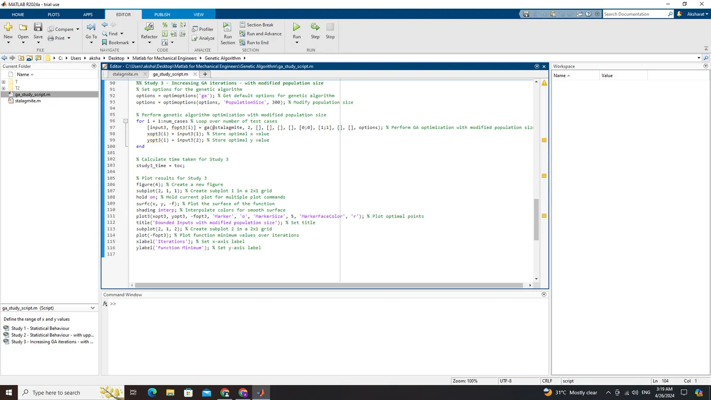
%% Study 3 - Increasing GA iterations - with modified population size
% Set options for the genetic algorithm
options = optimoptions('ga'); % Get default options for genetic algorithm
options = optimoptions(options, 'PopulationSize', 300); % Modify population size

% Perform genetic algorithm optimization with modified population size
for i = 1:num_cases % Loop over number of test cases
    [input3, fopt3(i)] = ga(@stalagmite, 2, [], [], [], [], [0;0], [1;1], [], [], options); % Perform GA optimization with modified population size
    xopt3(i) = input3(1); % Store optimal x value
    yopt3(i) = input3(2); % Store optimal y value
end

% Calculate time taken for Study 3
study3_time = toc;

% Plot results for Study 3
figure(4); % Create a new figure
subplot(2, 1, 1); % Create subplot 1 in a 2x1 grid
hold on; % Hold current plot for multiple plot commands
surfc(x, y, -f); % Plot the surface of the function
shading interp; % Interpolate colors for smooth surface
plot3(xopt3, yopt3, -fopt3, 'Marker', 'o', 'MarkerSize', 5, 'MarkerFaceColor', 'r'); % Plot optimal points
title('Bounded Inputs with modified population size'); % Set title
subplot(2, 1, 2); % Create subplot 2 in a 2x1 grid
plot(-fopt3); % Plot function minimum values over iterations
xlabel('Iterations'); % Set x-axis label
ylabel('Function Minimum'); % Set y-axis label

Explanation:

Data Generation

x = linspace(0, 0.6, 150);
y = linspace(0, 0.6, 150);

These lines generate vectors x and y, each containing 150 equally spaced points ranging from 0 to 0.6. These vectors represent the range of values for the variables x and y.

Meshgrid Creation

[xx, yy] = meshgrid(x, y);

The meshgrid function creates a grid of points by combining the x and y vectors. It generates two matrices, xx and yy, where each element of xx corresponds to a specific x value and each element of yy corresponds to a specific y value. Together, xx and yy define a meshgrid of points in the (x, y) plane.

Initialize Matrix To Store Function Values

f = zeros(length(xx), length(yy));

Here, a matrix f is initialized to store the function values calculated at each point in the meshgrid. It is preallocated with zeros to match the dimensions of the meshgrid, ensuring efficient memory usage and faster computation.

Calculate Function Values for Each Point in the Meshgrid

for i = 1:length(xx)
    for j = 1:length(yy)
        input_vector(1) = xx(i, j);
        input_vector(2) = yy(i, j);
        f(i, j) = stalagmite(input_vector);
    end
end

These nested loops iterate over each point in the meshgrid. At each iteration, the current x and y coordinates are used to create an input vector, which is then passed to the stalagmite function to calculate the corresponding function value. This value is stored in the f matrix.

Plot of Function Surface

figure(1);
surf(x, y, -f);
shading interp;
xlabel('X');
ylabel('Y');
title('Surface Plot of Stalagmite Function');

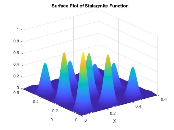
The figure(1) creates a surface plot of the "stalagmite" function using MATLAB. It plots the function values over the range of x and y values, adjusting the appearance of the plot for clarity by interpolating colors. Additionally, it labels the axes as "X" and "Y" and sets the title of the plot to "Surface Plot of Stalagmite Function" to provide context for the plotted data.

Number of Test Cases

num_cases = 50;

This line defines the variable num_cases, specifying the number of test cases to be conducted in each study. In this case, it's set to 50, meaning each optimization algorithm will be run 50 times to assess its performance statistically.

Study 1: Genetic Algorithm Optimization without Bounds

for i = 1:num_cases
    [input1, fopt1(i)] = ga(@stalagmite, 2);
    xopt1(i) = input1(1);
    yopt1(i) = input1(2);
end

In this study, the genetic algorithm optimization is performed without bounds for a specified number of test cases (num_cases). Each iteration optimizes the stalagmite function with two input variables. The optimal input values and corresponding function values are stored in xopt1, yopt1, and fopt1.

Study 1 Time

% Time the first study
tic;

% Remaining part of the code for Study 1

% Calculate time taken for Study 1
study1_time = toc;

The tic and toc functions are used to measure the time taken for the execution of this study, and the elapsed time is stored in the variable study1_time.

Plotting the Results for Study 1

figure(2);
subplot(2, 1, 1);
hold on;
surfc(x, y, -f);
shading interp;
plot3(xopt1, yopt1, -fopt1, 'Marker', 'o', 'MarkerSize', 5, 'MarkerFaceColor', 'r');
title('Unbounded Inputs');
subplot(2, 1, 2);
plot(-fopt1);
xlabel('Iterations');
ylabel('Function Minimum');

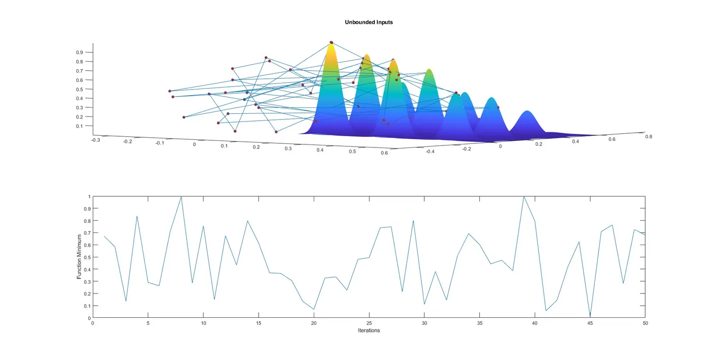
In the second plot (figure(2)), there are two subplots:

1. Surface Plot with Optimal Points: The upper subplot displays the surface of the stalagmite function similar to the first plot. Additionally, it marks the optimal points found by the genetic algorithm optimization without bounds. These points are represented by red markers on the surface plot, indicating where the algorithm converged to find optimal solutions.
2. Function Minimum over Iterations: The lower subplot shows how the function minimum value changes over the iterations of the genetic algorithm optimization. It plots the function minimum against the number of iterations, providing insights into the convergence behavior of the optimization algorithm.

Study 2: Genetic Algorithm Optimization with Bounds

for i = 1:num_cases
    [input2, fopt2(i)] = ga(@stalagmite, 2, [], [], [], [], [0;0], [1;1]);
    xopt2(i) = input2(1);
    yopt2(i) = input2(2);
end

Similar to Study 1, this study employs the genetic algorithm, but with bounds set on the input variables. The algorithm is constrained to search within the specified upper and lower bounds for each input variable. The optimal solutions and corresponding function values are recorded for further analysis.

Study 2 Time

% Time the second study
tic;

% Remaining part of the code for Study 2

% Calculate time taken for Study 2
study2_time = toc;

The tic and toc functions are used to measure the time taken for the execution of this study, and the elapsed time is stored in the variable study2_time.

Plotting the Results for Study 2

figure(3);
subplot(2, 1, 1);
hold on;
surfc(x, y, -f);
shading interp;
plot3(xopt2, yopt2, -fopt2, 'Marker', 'o', 'MarkerSize', 5, 'MarkerFaceColor', 'r');
title('Bounded Inputs');
subplot(2, 1, 2);
plot(-fopt2);
xlabel('Iterations');
ylabel('Function Minimum');

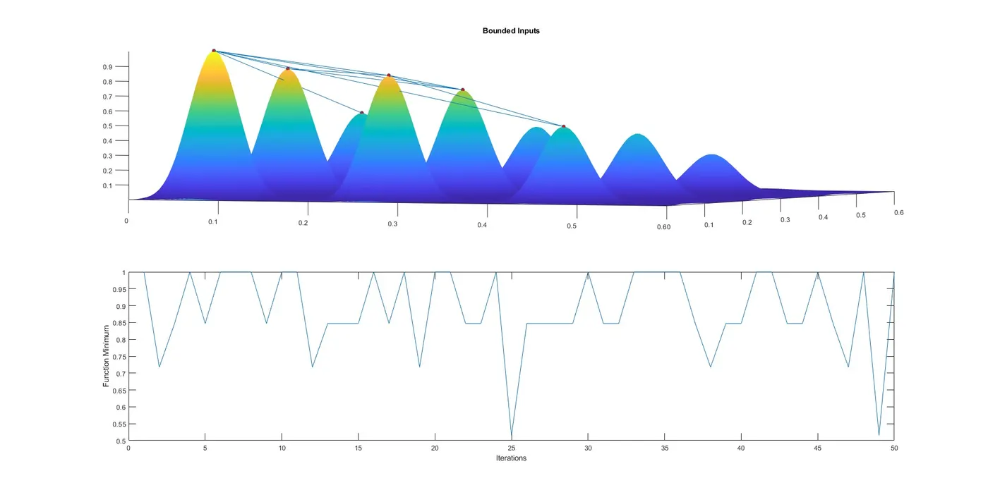
Similar to the second plot, this plot (figure(3)) also contains two subplots:

1. Surface Plot with Optimal Points: The upper subplot displays the surface of the stalagmite function with optimal points found by the genetic algorithm optimization with bounds. Similar to the previous plot, these points are represented by red markers on the surface plot.
2. Function Minimum over Iterations: The lower subplot shows how the function minimum value changes over the iterations of the genetic algorithm optimization with bounds. This plot allows comparison of convergence behavior between optimization with and without bounds.

Study 3: Genetic Algorithm Optimization with Modified Population Size

options = optimoptions('ga');
options = optimoptions(options, 'PopulationSize', 170);

for i = 1:num_cases
    [input3, fopt3(i)] = ga(@stalagmite, 2, [], [], [], [], [0;0], [1;1], [], [], options);
    xopt3(i) = input3(1);
    yopt3(i) = input3(2);
end

This study aims to investigate the effect of modifying the population size in the genetic algorithm. The algorithm options are configured to increase the population size to 300 individuals. The genetic algorithm is then executed num_cases times, and the optimal solutions along with their corresponding function values are recorded for analysis.

Study 3 Time

% Time the second study
tic;

% Remaining part of the code for Study 3

% Calculate time taken for Study 3
study3_time = toc;

The tic and toc functions are used to measure the time taken for the execution of this study, and the elapsed time is stored in the variable study3_time.

Plotting the Results for Study 3

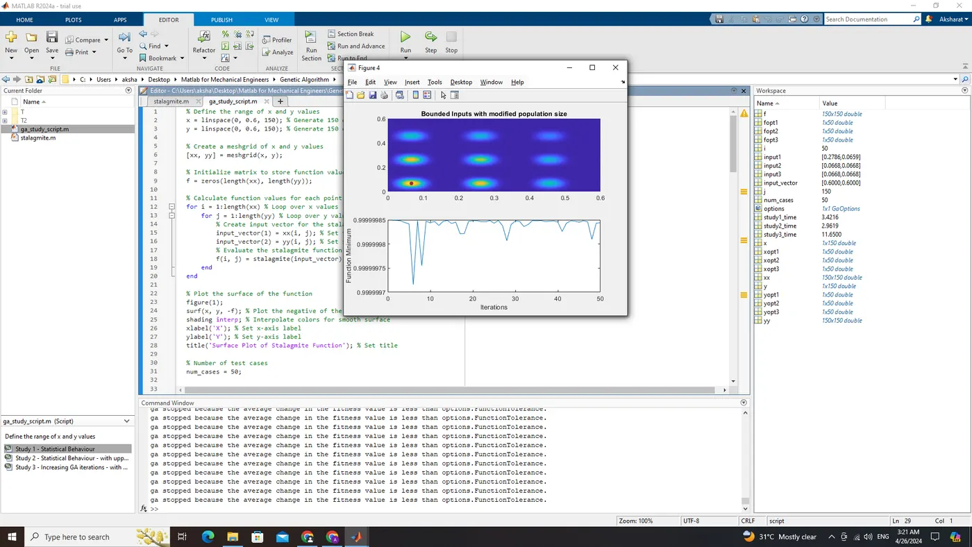
figure(4);
subplot(2, 1, 1);
hold on;
surfc(x, y, -f);
shading interp;
plot3(xopt3, yopt3, -fopt3, 'Marker', 'o', 'MarkerSize', 5, 'MarkerFaceColor', 'r');
title('Bounded Inputs with modified population size');
subplot(2, 1, 2);
plot(-fopt3);
xlabel('Iterations');
ylabel('Function Minimum');

In the fourth plot (figure(4)), there are also two subplots:

1. Surface Plot with Optimal Points: The upper subplot displays the surface of the stalagmite function with optimal points found by the genetic algorithm optimization with a modified population size. Once again, these points are represented by red markers on the surface plot.
2. Function Minimum over Iterations: The lower subplot shows how the function minimum value changes over the iterations of the genetic algorithm optimization with the modified population size. This plot allows comparison of convergence behavior between different population sizes.

Overall Interpretation

These plots provide a comprehensive visualization of the stalagmite function, along with the optimization process under various conditions. They help in understanding how different factors, such as input bounds and population size, affect the performance of the genetic algorithm in finding optimal solutions. By examining these plots, one can gain insights into the behavior of the optimization algorithm and make informed decisions about parameter tuning and optimization strategies.

Output:

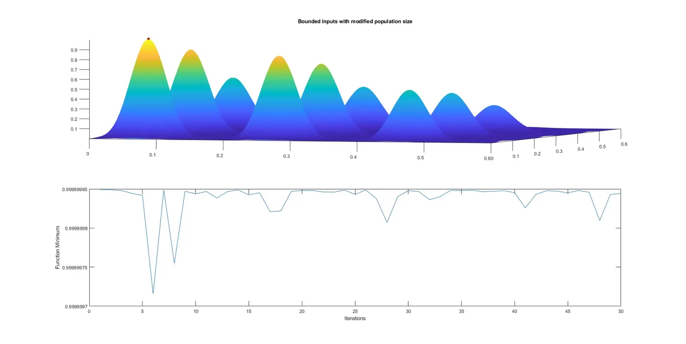
From the fopt3 array, the highest value is approximately -0.999999715971872.

So, the global maximum of the objective function (the minimum of the negative objective function) is approximately 0.999999715971872 ~ 1.00000

Study 1: Unbounded Inputs

• In this study, the genetic algorithm optimization is performed without any bounds on the input variables.
• The code conducts 50 test cases, optimizing the function stalagmite with two input variables.
• The optimization results are plotted in two subplots:
  1. The surface plot of the function overlaid with the optimal points found by the GA.
  2. The convergence plot showing how the minimum function value changes over iterations.

Study 2: Bounded Inputs

• This study is similar to Study 1 but with the addition of upper and lower bounds on the input variables.
• The bounds are set to [0, 1] for both variables.
• Again, 50 test cases are conducted.
• The plots are similar to Study 1 but for the bounded optimization.

Study 3: Increasing GA Iterations with Modified Population Size

• Here, the code explores the effect of modifying the population size in the genetic algorithm.
• The default population size for the GA is overridden to 300.
• 50 test cases are conducted again.
• The plots are similar to the previous studies but for the modified population size.

Observations:

• Study 1 vs. Study 2: Comparing the results between unbounded and bounded inputs, we might observe differences in convergence rates and final solutions due to the imposition of bounds. Bounded optimization may lead to solutions that lie within the specified range, which could differ from the unconstrained optimum.
• Study 2 vs. Study 3: By increasing the population size in Study 3, we might observe changes in convergence speed and possibly better solutions due to a larger exploration of the search space. This could lead to finding more globally optimal solutions or avoiding local optima.

The effectiveness of these strategies can be evaluated based on factors such as convergence speed, solution quality, and computational cost. Additionally, further analysis, such as sensitivity studies or comparisons with other optimization techniques, could provide deeper insights into the behavior of the genetic algorithm for this specific problem.

Conclusion:

• The code successfully demonstrates the application of GA optimization techniques to the stalagmite function under various conditions.
• Optimization with bounded inputs ensures solutions within defined constraints, while increasing GA iterations with modified population size can enhance optimization performance.
• The study provides insights into the behavior of GA optimization algorithms and their effectiveness in solving constrained optimization problems.