Week 5 - Genetic Algorithm

OBJECTIVE :- To write a MATLAB code on Genetic Algorithm.

PROBLEM STATEMENT :-

Try to understand the concept of GA by reffering to various sources before you attend this challenge. Look out for information regarding stalagmite function and ways to optimize it.

• Write a code in MATLAB to optimize the stalagmite function and find the global maxima of the function
• Clearly explain the concept of GA in our own words and also explain the syntax for ga in MATLAB in our report.
• Make sure that our code gives the same output, even if it is made to run several times.
• Plot graphs for all 3 studies and for F maximum verses no. of iterations. Title and axes labels are a must, legend could be shown if necessary.

Content expected in the report-

1. Step wise explaination of your code
2. Mention the error while programming
3. steps taken to overcome those errors
4. Screenshot showing errors thrown in command window

THEORY & INTRODUCTIONS :-

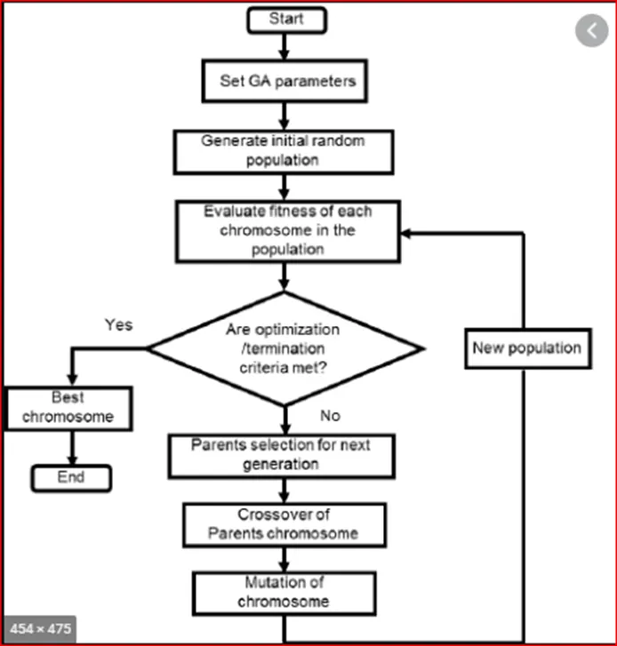
The genetic algorithm is inspired by the process that drives biological evaluation. The process of evaluation starts with the selection of fittest individuals from a population. Then they produce offspring which inherrit the charecterastics of the parents and will be added to the next generation. If parents have better fitness, their offspring will be better than parents and have a better chance at surviving. This process keeps on iterating and at the end, a generation with the fittest individuals will be found. And this is the main working principle for the algorithm because at each step, the genetic algorithm selects randomly from the current populations tobe parents and uses them to produce the children forthe next geeratio.Over successive generations, the population evolves towards an optimal solution. The genetic algorithm can be applied to solve a variety of optimization problems that are not well suited for standard optiization algorith, including problems i which the objective function is discontinuous, nondifferentiable, stachastic or highly nonlinear.

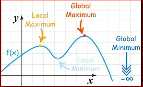
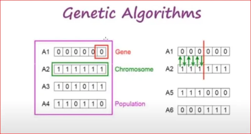
A genetic algorithm uses three main types of rules at each step to create the next generation from the current population:Selection rules select individuals, called parents, that contribute to populations in the next generation.
Crossover rules combine two parents to create children for future generations.
Mutation rules apply random changes to individual parents to create children.

Algorithm working sequence:-

The algorithm then creates a sequence of new populations. At each step, the algorithm uses individuals in the current generation to create the next population. It uses the fitness function to create a new population, which is the function you want to optimize. In standard optimization algorithms, this function is known as the objective function. The toolkit software tries to find the minimum fitness function.

The algorithm performs the following steps −

• The algorithm starts by creating random initial populations.It then scales the raw fitness scores to convert them into a more usable range of values. These scaled values ​​are called expectation values.
• It then selects members, called parents, based on their expectations.
• Along with individuals who have high fitness, some individuals in the current population who have lower fitness are selected as elite. These elite individuals are passed on to other populations. It also creates children by random changes in the mutation of one parent or by combining the vector records of a pair of parent crosses.
• They then replace the current population with children to create the next generation.
• It then evaluates each member of the current population by calculating its fitness value. These values ​​are called raw fitness scores then the algorithm stops when one of the stopping criteria is met.

Input Function:

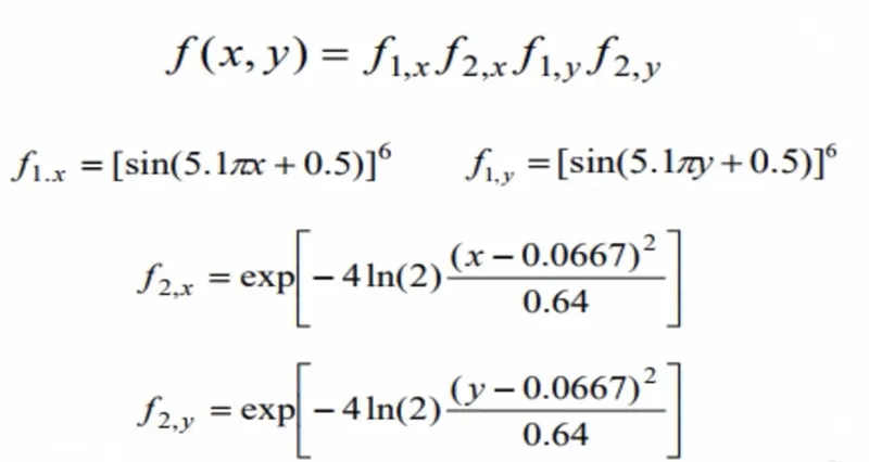
Code:

% A program to study the performance of the Genetic Algorithm (GA) for optimizing the "stalagmite" function.

clear all
close all
clc

% Define the domain of the function
x = linspace(0, 0.6, 150);
y = linspace(0, 0.6, 150);
[xx, yy] = meshgrid(x, y);

% Evaluate the Stalagmite function for the 2D mesh
for i = 1:length(xx)
    for j = 1:length(yy)
        input_value(1) = xx(i, j);
        input_value(2) = yy(i, j);
        f(i, j) = stalagmite(input_value);
    end
end

num_cases = 50;

% Study1: Unbounded statistical behavior
tic
for i = 1:num_cases
    [inputs1, fopt1(i)] = ga(@stalagmite, 2);
    xopt1(i) = inputs1(1);
    yopt1(i) = inputs1(2);
end
study1_time = toc;

% Study2: Bounded statistical behavior
tic
for i = 1:num_cases
    [inputs2, fopt2(i)] = ga(@stalagmite, 2, [], [], [], [], [0; 0], [1; 1]);
    xopt2(i) = inputs2(1);
    yopt2(i) = inputs2(2);
end
study2_time = toc;

% Study3: Bounded statistical behavior with modified population size
options = optimoptions('ga', 'PopulationSize', 170);
tic
for i = 1:num_cases
    [inputs3, fopt3(i)] = ga(@stalagmite, 2, [], [], [], [], [0; 0], [1; 1], [], [], options);
    xopt3(i) = inputs3(1);
    yopt3(i) = inputs3(2);
end
study3_time = toc;

Total_time = study1_time + study2_time + study3_time;

% Plots for each study
figure(1)
subplot(2, 1, 1)
hold on
surfc(xx, yy, -f)
xlabel('X-Values')
ylabel('Y-Values')
zlabel('Function Values')
shading interp
plot3(xopt1, yopt1, -fopt1, 'marker', 'o', 'markersize', 5, 'markerfacecolor', 'r')
title('Unbounded Statistical Behavior')
subplot(2, 1, 2)
plot(-fopt1)
xlabel('Iterations')
ylabel('Function maximum')

figure(2)
subplot(2, 1, 1)
hold on
surfc(xx, yy, -f)
xlabel('X-Values')
ylabel('Y-Values')
zlabel('Function Values')
shading interp
plot3(xopt2, yopt2, -fopt2, 'marker', 'o', 'markersize', 5, 'markerfacecolor', 'r')
title('Bounded Statistical Behavior')
subplot(2, 1, 2)
plot(-fopt2)
xlabel('Iterations')
ylabel('Function Maximum')

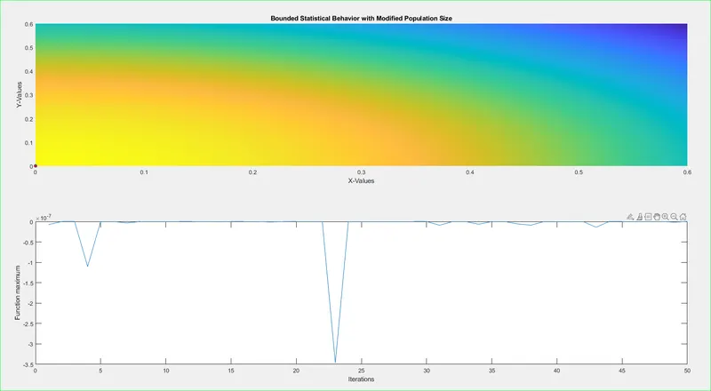
figure(3)
subplot(2, 1, 1)
hold on
surfc(xx, yy, -f)
xlabel('X-Values')
ylabel('Y-Values')
zlabel('Function Values')
shading interp
plot3(xopt3, yopt3, -fopt3, 'marker', 'o', 'markersize', 5, 'markerfacecolor', 'r')
title('Bounded Statistical Behavior with Modified Population Size')
subplot(2, 1, 2)
plot(-fopt3)
xlabel('Iterations')
ylabel('Function maximum')

% Results and summary
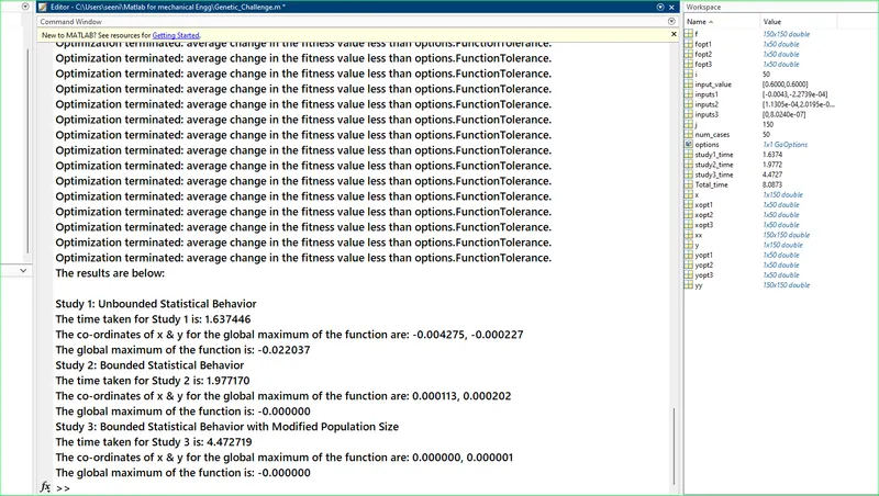
fprintf('The results are below:\n\n');

fprintf('Study 1: Unbounded Statistical Behavior\n');
fprintf('The time taken for Study 1 is: %f\n', study1_time);
fprintf('The co-ordinates of x & y for the global maximum of the function are: %f, %f\n', inputs1(1), inputs1(2));
fprintf('The global maximum of the function is: %f\n', -(mean(fopt1)));

fprintf('Study 2: Bounded Statistical Behavior\n');
fprintf('The time taken for Study 2 is: %f\n', study2_time);
fprintf('The co-ordinates of x & y for the global maximum of the function are: %f, %f\n', inputs2(1), inputs2(2));
fprintf('The global maximum of the function is: %f\n', -(mean(fopt2)));

fprintf('Study 3: Bounded Statistical Behavior with Modified Population Size\n');
fprintf('The time taken for Study 3 is: %f\n', study3_time);
fprintf('The co-ordinates of x & y for the global maximum of the function are: %f, %f\n', inputs3(1), inputs3(2));
fprintf('The global maximum of the function is: %f\n', -(mean(fopt3)));

% Define the 'stalagmite' function
function result = stalagmite(input_values)
    x = input_values(1);
    y = input_values(2);
    result = x^2 + y^2; % Replace this with your actual function
end

% Rest of the code (loading data and GA optimization) remains the same

Result Images:

Figure 1:

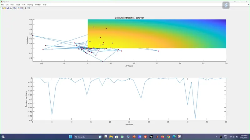
Figure 2:

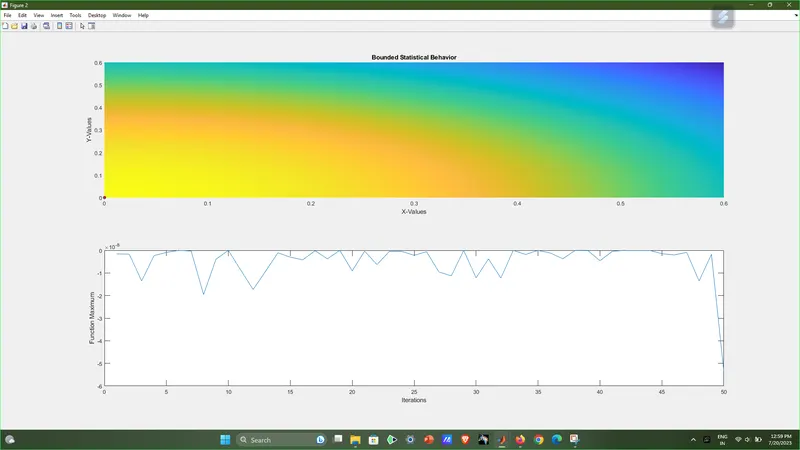
Figure 3:

Code Output:

Explanation:

• First, the Linspace command is used to define x & y with 150 elements between zero and 0.6 inclusive of boundaries.
• It then sets num_cases to be used as the iteration counter to 50 then a 2D grid is created using the meshgrid command is created from input x & y to be output to xx & yy then a for loop is used to solve the genetic algorithm for each element in the 2D mesh grid.
• The length of rows and columns (which have the same length) are used as counters then the input vector is declared as ga requires the input vector, which is each value in the mesh grid the output of the stalagmite function is then stored in a matrix.
• Then the tic command is used to start the timer then a for loop bounded by the number of iterations is created.then the ga code is entered for an unrestricted statistical study, which has the following format:
• [inputs, fopt] = ga(fun, nvars)
• inputs represent the x & y parameter values ​​for which the function has the smallest value (fopt)
• fun - function to optimize, in this case stalagmite
• nvars - number of design variables, in this case only x and y are the variables to be plotted
• Then the output is the smallest (minimum) value of the function for each iteration and its x & y coordinates, which are stored in separate variables
• then the 'toc' command is used to stop the timer and the output is stored in study_time1
• then figure 1 is plotted as per following steps -
• The first subplot statement is used to split the plot window so that more than one plot can be drawn in the same window, two rows and one column are specified, and then the position of each plot is selected
• then a hold on command is used to prevent the chart from being deleted
• surfc command is used to plot contour with xx & yy value from mesh grid as input and negative optimal value is used as we need to maximize function,then the x, y and z axes are marked.
• The interp shading is used to smooth the feature rendering and remove the grid lines
• then the plot 3 command is used to plot the point in 3D, here it will be plotfopt because we need the maximum value of the function, not the minimum,then the chart name is selected
  then the value of the fopt function is plotted on the second graph in the second row then its x & y axis are labeled.then the same study is performed, but this time it is bounded (has a lower and upper limit), which requires the same commands and step except for the ga command, which has the following format:
• [input, fopt] = ga(fun, nvars, A, b, Aeq, beq, lb, ub)
• Inputs, fopt, entertainment and nvars are same as study-1
• A - Linear inequality constraint: real matrix if none then []
• b - Linear inequality constraint: real vector if none then []
• Aeq - Linear equality constraint - :- real matrix if none then []
• beq - Linear Equality Constraints - real vector if not then []
• lb - lower bound, specified as a real vector or array
• ub - upper bound, specified as a real vector or array
• the scope of the genetic algorithm is bounded by introducing values ​​for the lower and upper bounds and thus the values ​​of the global maxima and the values ​​of x & y will be in the defined search space in the inputs
  then a study of increasing population size was done which is the same as before but had a different ga code:
• [inputs, fopt] = ga(fun, nvars, A, b, Aeq, beq, lb, ub, nonlcon, IntCon, options)
• inputs, fopt, fun and nvars, A, b, Aeq, beq, lb, ub are same as study-1 and study-2 respectively
• nonlcon - non-linear constraints specified as a function handle or function name. If none then []
• IntCon - Integer variables specified as a vector of positive integers if none then []
• Options - Optimization options, specified as the output of an optimization option or structure.
• The range of the genetic algorithm is limited as in study-2, but command options are introduced to increase the population size to improve accuracy then the total time is calculated,then using the fprintf command the results are printed in command windows
• Then the study time is printed and the x, y coordinates of the maximum optimal values ​​are printed,So print the optimal values ​​of the function (maximum value) which is calculated from (the negative average of) all iterations of the output value and use the negative sign to get the maximum value.
• Therefore the study time of the entire 3 studies together is printed.