Week 5 - Genetic Algorithm

AIM: Program in MATLAB to find the global maxima and optimise the stalagmite function using syntax ga which is in-built in MATLAB.

OBJECTIVE:

• Program in MATLAB to optimise the stalagmite function and find the global maxima of the function.
• Clearly expalin the concept of genetic algorithm in your own words and also explain the syntax for ga in MATLAB in your report.
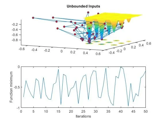
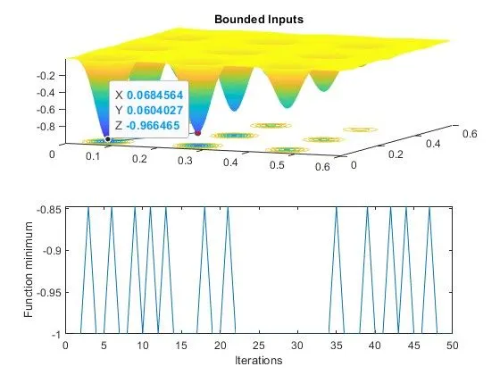
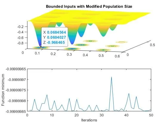
• Plot graphs for all 3 studies and for F maximum vs no. of iterations. Title and axes labels are a must, legends could be shown if necessary.

THEORY:

Genetic Algorithm (GA) is a search-based optimisation technique based on principles of genetics and natural-selection. It's frequently used to find the optimal and near-optimal solutions. It's mainly used to solve optimisation problem, in machine learning, etc.

GA follows the follwing process:

• Initialisation
• Selection
• Cross-Over
• Mutation

What is Stalagmite:

A stalagmite is a type of rock formation that rises from the floor of a cave due to the accumulation of material deposited on the floor from ceiling drippings. In this program, we will create a function which will create a 3D graph to plot stalagmite-like structure in that graph. The graph will follow the equation(f(x,y)) given below,

`f(x,y)=f_(1,x)f_(2,x)f_(1,y)f_(2,y)` where

`f_(1,x)=[sin(5.1pix+0.5)]^6`,

`f_(1,y)=[sin(5.1piy+0.5)]^6``,

`f_(2,x)=exp[-4ln(2)(x-0.0667)^2/0.64]` and

`f_(2,y)=exp[-4ln(2)(y-0.0667)^2/0.64]`

PROGRAM:

Program to find the stalagmite structure by formulating the equation given above:

function s = stalagmite_func(input_vector)

x = input_vector(1);
y = input_vector(2);

f1 = (sin(5.1*pi*x+0.5))^6;
f2 = (sin(5.1*pi*y+0.5))^6;
f3 = exp((-4*log(2)*(x-0.0667)^2)/0.64);
f4 = exp((-4*log(2)*(y-0.0667)^2)/0.64);

s = -(f1*f2*f3*f4); %Negative sign used to show downward depression

end

EXPLANATION:

This program has 9 lines. The line by line explanation is given below:

1) function s = stalagmite_func(input_vector): To declare a function loop 'stalagmite_func()' that accepts an array 'input_vector' and returns output in 's'.

2) x = input_vector(1);: To declare a variable 'x' that stores the first row values of 'input_vector' inside 'x'

3) y = input_vector(2);: To declare a variable 'y' that stores the first row values of 'input_vector' inside 'y'

4) f1 = (sin(5.1*pi*x+0.5))^6;: To declare a variable `f_(1,x)`.

5) f1 = (sin(5.1*pi*y+0.5))^6;:To declare a variable `f_(1,y)`.

6) f3 = exp((-4*log(2)*(x-0.0667)^2)/0.64);:To declare a variable `f_(2,x)`.

7) f3 = exp((-4*log(2)*(y-0.0667)^2)/0.64);:To declare a variable `f_(2,y)`.

8) s = -(f1*f2*f3*f4);: T declare a variable `f` of stalagmite function mentioned in function loop as 's'. Negative sign used to show downward depression.

9) end: To end the function loop.

Program to find the global maxima and optimise the stalagmite function using syntax ga:

clear all
close all
clc

% Defining our Search space
x = linspace(0,0.6,150);
y = linspace(0,0.6,150);
num_cases = 50;

% Creating a 2D mesh
[X Y] = meshgrid(x,y);

% Evaluating the Stalagmite function
for i = 1:length(X)
    for j = 1:length(Y)
        input_vector(1) = X(i,j);
        input_vector(2) = Y(i,j);
        s(i,j) = stalagmite_func(input_vector);
    end
end

surfc(X,Y,s)
xlabel('X-axis value')
ylabel('Y-axis value')
zlabel('Z-axis value')

%shading interp

[inputs, fval] = ga(@stalagmite_func,2)

% Study 1 - Statistical Behaviour:
tic
for i=1:num_cases
    [inputs,fopt(i)]=ga(@stalagmite_func,2);
    xopt(i)=inputs(1);
    yopt(i)=inputs(2);
end

study1_time = toc; 

figure(1)
subplot(2,1,1)
hold on
surfc(x,y,s)
shading interp
plot3(xopt,yopt,fopt,'marker','o','markersize',5,'markerfacecolor','r')
title('Unbounded Inputs')
subplot(2,1,2)
plot(fopt)
xlabel('Iterations');
ylabel('Function minimum');

tic
% Study 2 - Statistical behaviour - with upper and lower bounds
for i=1:num_cases
    [inputs,fopt(i)]=ga(@stalagmite_func,2,[],[],[],[],[0;0],[0.6;0.6]);
    xopt(i)=inputs(1);
    yopt(i)=inputs(2);
end
study2_time=toc;

figure(2)
subplot(2,1,1)
hold on
surfc(x,y,s)
shading interp
plot3(xopt,yopt,fopt,'marker','o','markersize',5,'markerfacecolor','r')
title('Bounded Inputs')
subplot(2,1,2)
plot(fopt)
xlabel('Iterations');
ylabel('Function minimum');

% Study 3 - Increasing GA Iterations
options=optimoptions('ga');
options=optimoptions(options,'PopulationSize',200);

tic
for i=1:num_cases
    [inputs,fopt(i)]=ga(@stalagmite_func,2,[],[],[],[],[0;0],[0.6;0.6],[],[],options);
    xopt(i)=inputs(1);
    yopt(i)=inputs(2);
end
study3_time=toc;

figure(3)
subplot(2,1,1)
hold on
surfc(x,y,s)
shading interp
plot3(xopt,yopt,fopt,'marker','o','markersize',5,'markerfacecolor','r')
title('Bounded Inputs with Modified Population Size')
subplot(2,1,2)
plot(fopt)
xlabel('Iterations');
ylabel('Function minimum');

EXPLANATION:

This program has 75 lines. The line by line explanation is given below:

1) clear all: This is a command that is used to clear all workspace data.

2) close all: This is a command that is used to close any plot/graphs.

3) clc: This is a clear screen command. It clears command box.

4) x = linspace(0,0.6,150);: To create an array 'x' from 0 to 0.6 with 150 divisions.

5) y = linspace(0,0.6,150);: To create an array 'y' from 0 to 0.6 with 150 divisions.

6) num_cases = 50;: To run the GA 50 times, variable 'num_cases' is used in respectable for loop.

7) [X Y] = meshgrid(x,y);: To returns 2-D grid coordinates based on the coordinates contained in vectors x and y. X is a matrix where each row is a copy of x, and Y is a matrix where each column is a copy of y. The grid represented by the coordinates X and Y has length(y) rows and length(x) columns.

8) for i = 1:length(X): Start of nested for loop to evaluate stalagmite function to take 'X'.

9) for j = 1:length(Y): Start of nested for loop to evaluate stalagmite function to take 'Y'.

10) input_vector(1) = X(i,j);: To declare variable that stores x values that is in first row of matrix 'X'.

11) input_vector(2) = Y(i,j);: To declare variable that stores x values that is in first row of matrix 'Y'.

12) s(i,j) = stalagmite_func(input_vector);: To declare array that stores stalagmite function which evaluates input_vector(1) and input_vector(2).

13) end: To end the 2nd nested for loop

14) end: To end the 1st nested for loop.

15) - 19): To plot the stalagmite structure in a 3D graph, which is not shown and replaced by 1st subplot.

20) tic: Starting of timer is used to measure how long it takes to study the iterations.

21) for i=1:num_cases: For loop to start to studying the statistical behaviour for 1st study.

22) [inputs,fopt(i)]=ga(@stalagmite_func,2);: Variables to store the stalagmite function and number of variables inside fopt(i).

23) xopt(i)=inputs(1);: Array that stores x values from 'input' matrix.

24) yopt(i)=inputs(2);: Array that stores y values from 'input' matrix.

25) end: To end the for loop

26) study1_time = toc;: Ending of timer to measure how long it takes to study the iterations and to store inside the variable 'study1_time' for 1st iteration.

27) figure(1): To start a figure showing two graphs one is 3D and another is 2D depicting minimum value of function VS number of iterations.

28) subplot(2,1,1): To start 1st subplot showing 2 graphs mentioned above. It divides the current figure into an 2-by-1 grid and creates axes in the position specified by 1.

29) hold on: To retains plots in the current axes so that new plots added to the axes do not delete existing plots.

30) surfc(x,y,s): To create a three-dimensional surface plot with the the values in matrix 's' as heights above a grid in the x-y plane defined by x and y.

31) shading interp: To show interpolated shading. It varies the color in each line segment and face by interpolating the colormap index or true color value across the line or face.

32) plot3(xopt,yopt,fopt,'marker','o','markersize',5,'markerfacecolor','r'): To plot coordinates in 3D space by specifying xopt, yopt and fopt using marker, markersize and markerfacecolor.

33) title('Unbounded Inputs'): To mention a title of 3D graph as "Unbounded Inputs".

34) subplot(2,1,2): To start 2nd subplot showing 2 graphs mentioned above. It divides the current figure into an 2-by-1 grid and creates axes in the position specified by 2.

35) plot(fopt): To plot an array 'fopt' explained in first for loop.

36) xlabel('Iterations');: To label the graph X-axis as "Iterations".

37) ylabel('Function minimum');: To label the graph Y-axis as "Function minimum".

38) tic: Starting of timer is used to measure how long it takes to study the iterations.

39) for i=1:num_cases: For loop to start to studying the statistical behaviour for 2nd study.

40) [inputs,fopt(i)]=ga(@stalagmite_func,2,[],[],[],[],[0;0],[0.6;0.6]);: To declare array that stores stalagmite function which evaluates input_vector(1) and input_vector(2). For no linear inequality constraints, [] is used instead. Then upper and lower limits of X and Y are noted as 0 and 0.6.

41) xopt(i)=inputs(1);: Array that stores x values from 'input' matrix.

42) yopt(i)=inputs(2);: Array that stores y values from 'input' matrix.

43) end: To end the for loop.

44) study2_time = toc;: Ending of timer to measure how long it takes to study the iterations and to store inside the variable 'study1_time' for 2nd iteration.

45) figure(2): To start the 2nd figure showing two graphs one is 3D and another is 2D depicting minimum value of function VS number of iterations.

46) - 55) : Same explanation as line 28) - 37) but the 'title' of 3D graph is "Bounded Inputs".

56) options=optimoptions('ga');: Variable returns a set of default options for the solver named 'ga' used for optimization solution.

57) options=optimoptions(options,'PopulationSize',200);: Variable returns options with specified parameters set using population size of 200.

58) tic: Starting of timer is used to measure how long it takes to study the iterations.

59) for i=1:num_cases: For loop to start to studying the statistical behaviour for 3rd study.

60) [inputs,fopt(i)]=ga(@stalagmite_func,2,[],[],[],[],[0;0],[0.6;0.6],[],[],options);: To declare array that stores stalagmite function which evaluates input_vector(1) and input_vector(2). For no linear inequality constraints, [] is used instead. Then upper and lower limits of X and Y are noted as 0 and 0.6. The linear inequalities of optimisation variables 'options' is also replaced by [].

61) xopt(i)=inputs(1);: Array that stores x values from 'input' matrix.

62) yopt(i)=inputs(2);: Array that stores y values from 'input' matrix.

63) end: To end the for loop.

64) study3_time = toc;: Ending of timer to measure how long it takes to study the iterations and to store inside the variable 'study1_time' for 2nd iteration.

65) figure(3): To start the 2nd figure showing two graphs one is 3D and another is 2D depicting minimum value of function VS number of iterations.

66) - 75): Same explanation as line 46) - 55) but the 'title' of 3D graph is "Bounded Inputs with Modified Population Size".

CONCLUSION:

1) The program ran succesfully.

2) The outputs shown below in 3 figures having 2 graphs each.

3) The time required to run the program is long which can be reduced by reducing the limits. Decreasing the population size will get more accurate results.

ERRORS FACED WHILE PROGRAMMING:

1) While NO errors were found in the command window, we had errors in the outputs.

2) In each for loop, the variable for ga was misunderstood and after further review later corrected.

3) The formulas for s in function loop was later given negative sign to see downward depression.

4) The subplot command was typed 'f' instead of 's' which was a big error.

OUTPUTS: