Week 4.1 - Solving second order ODEs
AIM: Write a program in MATLAB that can solves the ODE which represents the equation of motion of a simple pendulum with damping.
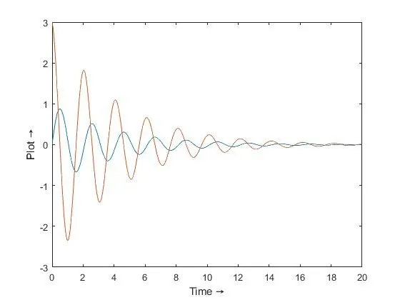
OBJECTIVE: To write a codes to create a graph of a plot and animation by introducing commands like ode45(). In this project we use function loop in seperate program to do the differenciation calculation and make an animation video for a simple pendulum and plot a graph of angular displacement and angular velocity VS Time graph:
THEORY:
In Engineering, ODE is used to describe the transient behavior of a system. A simple example is a pendulum
The way the pendulum moves depends on the Newtons second law. i.e.
`F = m*a = m*l*w^2` where'
`a = -g*sintheta` = acceleration of the simple pendulum
`T = 2(pi/omega)` = time period of the simple pendulum
When this law is written down, we get a second order Ordinary Differential Equation that describes the position of the "ball" w.r.t time.
Similarly, there are hundreds of ODEs that describe key phenomena and if you have the ability to solve these equations then you will be able to simulate any of theses systems.
FORMULA:
The position(theta) of the bob with respect to time of a simple pendulum can be determined by using the second order differential equations. The value theta can be solved by using the second order ODE and this can be achieved by breaking the higher order ODE i.e., second order ODE into no of first order ODE. The second order ode for simple pendulum will be as follows:
`(d^2theta)/dt^2+(b/m)d/dttheta+g/lsintheta` where
g = gravity in m/s^2,
L = length of the pendulum in m,
m = mass of the ball in kg,
b=damping coefficient.
Let `theta = theta_1`
Then `d/dttheta = d theta_1/dt = theta_2`
`(d^2theta)/dt^2 = (d^2theta_1)/dt^2 = d/dttheta_2`
From the ODE represents the equation of motion,
`d/dttheta_2 = -(b/m)theta2-(g/l)sintheta_1`
`d/dt[[theta_1],[theta_2]] = [[theta_2],[(-b/mtheta_2-g/lsintheta_1)]]`
The simple pendulum problem can be solved by using the second order ode functions and by solving these we will get the `theta_1` an `theta_2` values of the simple pendulum.
PROGRAM:
The program takes place in two forms :
1) Program for function named 'ode_func':
function [dtheta_dt] = ode_func(t,theta,b,g,l,m)

theta1 = theta(1);
theta2 = theta(2);
dtheta1_dt = theta2;
dtheta2_dt = -(b/m)*theta2 - (g/l)*sin(theta1);
dtheta_dt = [dtheta1_dt; dtheta2_dt];

end
EXPLANATION:
This program has 7 lines. The line by line explanation is given below:
1) function [dtheta_dt] = ode_func(t,theta,b,g,l,m): Function loop to declare function 'ode_func' which should take values of variables to evaluate a variable 'V' inside the loop.
2) theta1 = theta(1);: Variable that stores the 1st row value or the 1st value of theta. This process uses Runge-Kutta differentiation method.
3) theta2 = theta(2);: Variable that stores the 2nd row value or the 2nd value of theta.
4) dtheta1_dt = theta2;: Variable that stores value of `d/dttheta_1`from equation mentioned above.
5) dtheta2_dt = -(b/m)*theta2 - (g/l)*sin(theta1);: Variable that stores value of `d/dttheta_2`from equation mentioned above.
7) end: To end the function loop.
2) Program to creatwe animation and plotting:
clear all
close all
clc

b = 0.05; % damping coefficient.
g  = 9.81; % gravity in m/s^2
l = 1; % length of the pendulum in metres
m = 0.1; % mass of the ball in kg

%Initial Condition:
initial_condition = [0;3]; %in radians and rad/sec

%Time Points:
t_span = linspace(0,20,500); %in sec

%Solve ODE:
[t, results] = ode45(@(t,theta) ode_func(t,theta,b,g,l,m),t_span, initial_condition);

%Angular displacement and angular velocity VS Time graph:
figure(1)
plot(t,results(:,1))
hold on
plot(t,results(:,2))
ylabel('Plot →')
xlabel('Time →')

%Pendulum Loop:
ct = 1;
theta = results(:,1);
for i = 1 : length(theta)
    angle = theta(i);
    figure(2)
    title('Simple Pendulum Animation:')
    x0 = 0;
    y0 = 0;
    x1 = -l*cos(((3*pi)/2)+angle);
    y1 = l*sin(((3*pi)/2)+angle);
    plot([x0 x1],[y0 y1],'LineWidth',4)
    hold on
    plot(x1,y1,'.','Markers',50,'Color','r')
    hold on
    plot([-2,2],[0,0],'LineWidth',5)
    hold off
    axis([-9,9,-4,4])
    pause(0.03)
    M(ct) = getframe(gcf);
    ct = ct + 1;
end

movie(M)
videofile = VideoWriter('Pendulum Animation.avi','Uncompressed AVI');
open(videofile)
writeVideo(videofile,M)
close(videofile)
EXPLANATION:
This program has 42 lines. The line by line explanation is given below:
1) clear all: This is a command that is used to clear all workspace data.
2) close all: This is a command that is used to close any plot/graphs.
3) clc: This is a clear screen command. It clears command box.
4) b = 0.05;: Variable that stores value of damping coefficient.
5) g = 9.81;: Variable that stores value of gravity in m/s^2.
6) l = 1;: Variable that stores value of length of the pendulum in m.
7) m = 0.1;: Variable that stores value of mass of the ball in kg.
8) initial_condition = [0;3];: Initial values of angular displacement=0 radians, angular velocity=3 rad/sec at time t=0 inside variable 'initial_condition'.
9) t_span = linspace(0,20,500);: Array to store the time values of timespan of oscillation between 0-20 seconds for 500 divisions.
10) [t, results] = ode45(@(t,theta) ode_func(t,theta,b,g,l,m),t_span, initial_condition);: A new in-built function ode45() used for evaluating ODE using 't', 'theta' and function named 'ode_func()' specified in another program mentioned previously, with initials 't_span' and 'initial_condition' inside array type variable [t, results].
11) figure(1): For two plottings in one graph or the 1st graph.
12) plot(t,results(:,1)): 1st plotting inside Time VS Plot graph.
13) hold on: To plot the second above first graph, hold on command is used.
14) plot(t,results(:,2)): 2nd plotting inside Time VS Plot graph.
15) ylabel('Plot →'): To label Y-axis as "Plot →".
16) xlabel('Time →'): To label X-axis as "Time →".
17) ct = 1;: Initial counter value is taken as 1. Counter is used to repeat the number of plots seperately for different outputs.
18) theta = results(:,1);: Value of theta mentioned in ode45() is stored.
19) for i = 1 : length(theta): For loop for doing iteration of plots inside one graph.
20) angle = theta(i);: Values of 'theta' is stored one by one inside variable 'angle' inside the loop.
21) figure(2): For many plottings in one graph or the 2nd graph.
22) title('Simple Pendulum Animation:'): To give title of the graph "Simple Pendulum Animation:".
23) x0 = 0;: Value of X-axis of 1st point is fixed in variable 'x0'.
24) y0 = 0;: Value of Y-axis of 1st point is fixed in variable 'y0'.
25) x1 =-l*cos(((3*pi)/2)+angle);: Value of X-axis for 2nd point for 'l' is fixed in variable 'x1'.
26) y1 = l*sind(((3*pi)/2)+angle);: Value of Y-axis for 2nd point for 'l' is fixed in variable 'y1'.
27) plot([x0 x1],[y0 y1],'LineWidth',4): To plot the length of pendulum 'l' with a width of 4.
28) hold on: To hold the plots of varying position of in one graph.
29) plot(x1,y1,'.','Markers',50,'Color','r'): To draw a ball of mass 'm' with size of 50.
30) hold on: To plot the fixed line above length graph, hold on command is used.
31) plot([-2,2],[0,0],'LineWidth',5): To plot the fixed line above length graph.
32) hold off: To set the hold state to off so that new plots added to the axes clear existing plots and reset all axes properties.
33) axis([-9,9,-4,4]): To fix the axes points.
34) pause(0.03): The time interval between consecutive graphs are taken as 0.03 seconds.
35) M(ct) = getframe(gcf);: All the graphs are stored inside the array 'M' with the help of command getframe() which captures axes or figure as movie frame.
36) ct = ct + 1;: Increaments the counter 'ct' by +1 inside nested for loop which stores the graphs as a frame in array 'M(ct)'.
37) end: To end the for loop.
38) movie(M): It plays the movie frames in array 'M' after collecting the fram 'videofile' stores the name of movie as 'Robot.avi' as 'Uncompressed AVI' in VideoWriter() command.
39) videofile = VideoWriter('Pendulum Animation.avi','Uncompressed AVI');: To publish/write a new video of a movie in movie() command.
40) open(videofile): Video mentioned in VideoWriter() command is opened with open() command.
41) writeVideo(videofile,M): It write video data to file stored in 'videofile'.
42) close(videofile): Created video closed after completion.
ERRORS FACED WHILE PROGRAMMING:
1) While NO errors were found in the command window, we had errors in the outputs.
2) In for loop, the vaue of angle used was not declared correctly for which the graph was not moving later corrected.
3) The formulas mentioned inside the for loop were initially typed wrong as a result animation was not correct.
4) The values of axis() was typed wrong and later corrected.
CONCLUSION:
1) The program ran succesfully.
2) The outputs shown below and as attachment and graph given below saved as Pendulum Animation.avi.
Graph for Time VS Plot:
Pendulum Animation:
https://drive.google.com/file/d/1FEdDcYOErLvgnrPIoJW_ImpSYQp1kIjf/view?usp=share_link