Week 5 - Genetic Algorithm
Report of Week 5 - Genetic Algorithm
Aim: Understanding the genetic algoritm and use of ga in matlab coding, and as per the goal we have to find the global maxima by optimising stalagmite function. As we know ga gives the minimum value by default figure out the way to find the global maxima in the stalagmite, and also values should be the same even after running it several times under 3 studies F maximum vs number of iteration.
Objective: 1) Should create a valid stalagmite function with the formula we have
`f(x,y) = f_(1,x) f_(2,x) f_(1,y) f_(2,y)`
`f_(1,x) = [sin(5.1pix + 0.5]^6`
`f_(1,y) = [sin(5.1piy+0.5)]^6`
`f_(2,x) = exp[-4ln(2)((x-0.0667)^2/0.64)]`
`f_(2,y) = exp[-4ln(2)((y-0.0667)^2/0.64)]`
2) create a code for optimising the stalagmite function by using a inbuilt solver ga.
3) As we know that ga gives the minima value as our main goal is to achieve the global maxima, hence figure out the way to do that.
4) After creating the code conduct 3 studies, 'Unbounded','Bounded', and 'Bounded with increasing iterations of ga'.
5) The objective of the same value to be achieved even after repeating many times.
6) Plot the graph with global maxima and plot a graph 'Function maximum' vs 'no of iteration'.
7) Submit the output results.
Theory part for better understanding
Genetic algorithm -> Before seeing what is genetic algorithm we should know the following.
1) What is optimisation?
2) What are the techniques available to perform optimisation?
3) What is GA?
4) How does GA works?
5) Where GA is used?
Solution
What is optimisation?
Optimisation is a decision making process, it helps to find the best results under a set of prioritized criteria or constraints. It is a procedure which is executed iteratively by comparing various solutions till an optimum or a satisfactory solution is found.
In other words.
Optimisation refers to the process of finding the best solution or set of solutions for a particular problem, given a set of constraints and objectives. The goal of optimization is to maximize or minimize a certain objective function while satisfying the constraints.
Optimisation can be applied to a wide range of fields, such as engineering, economics, computer science, and physics. In each of these fields, optimisation is used to find the best solutions to various problems, such as designing efficient structures, maximizing profits, optimizing algorithms, or minimizing waste.
2) What are the techniques available to perform optimisation?
There are two techniques available to perform optimisation.
1) Deterministic method: They are specific rules for moving one solution to another. In this technique, the output of the model is fully determined by the parameter values and the initial conditions.
Ex: Stress analysis of the component, this is a deterministic approach since the output results(stress values) fully depend on the initial conditions(loading condition) and the parameter values(force acting on the component and material properties).
2) Stochastic method: These are gaining popularity due to certain properties which deterministic algorithms do not possess. Stochastic models possess some inherent randomness, it is a probabilistic approach.
Ex: Varying the water paths from the mountain can vary the regional weather conditions, but the weather condition is not fully dependent on the water paths, hence there will be many statistical predictions to get the predictive model, since the weather condition depends on various factors such as solar distance, latitudinal location, air pressure, etc. Hence it is a predictive model.
The following is the procedure followed by any optimisation process
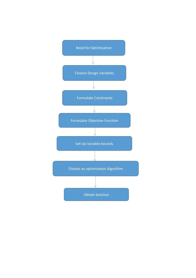
Let's understand the flowchart.
What are variables?
The parameters which you have to vary during the optimisation process are known as variables, Design dimensions can be varied to get the minimum stress.
What are constraints?
During the optimisation process, your output should not go beyond the certain limits, those are known as constraints. You can reduce the material used in such a way that the stress should not go beyond the ultimate stress of the material.
What is an objective function?
An objective function is as simple as a mathematical formula, which can be a predicted mathematical model that includes all the variable as input.
Ex: z=f(x,y) here the output(z) depends on the input variable (x&y).
What are variable bounds?
The variable bounds are the range of the input variables, that will be varied for every iteration to provide an optimised result.
Ex: The design variable (thickness)can be varied in the range between (5-7)mm, to get the minimum stress.
For choose an optimisation algorithm. We choose GA inbuilt solver.
What is GA?
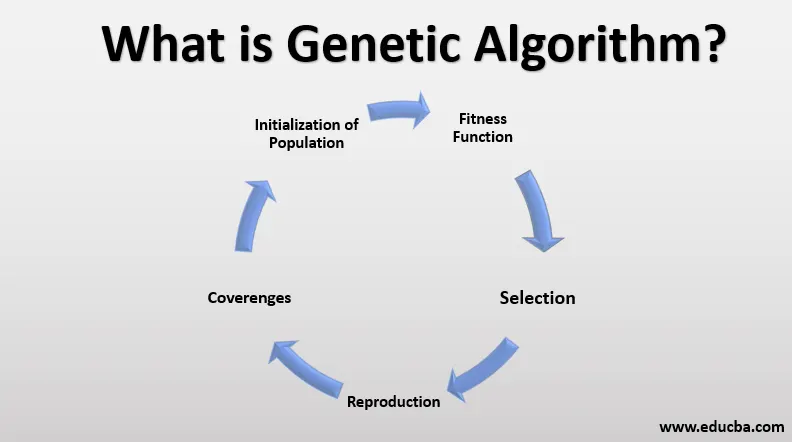
As shown above in the flowchart, we need to choose an optimisation algorithm to perform the optimisation optimisation process. Genetic algorithm is one of the optimisation processes.
Genetic Algorithm (GA) is a search based optimisation technique based on the principles of genetics and natural selection. It is frequently used to find optimal or near-optimal solutions.
It is frequently used to solve optimization problems, in research, and in machine learning.
How does GA work?
The following flow chart describes how the genetic algorithm works to find to find the optimal solution.
Applications of Genetic algorithm?
Genetic algorithms (GAs) are a type of evolutionary computation technique inspired by natural selection and genetics. They are used to solve optimization problems by mimicking the process of natural selection, crossover, and mutation. Here are some common applications of genetic algorithms:
- Optimization problems: Genetic algorithms are often used to optimize complex problems that cannot be solved using traditional optimization methods. These include optimization problems in engineering, economics, logistics, and other fields.
- Machine learning: Genetic algorithms can be used as a search technique to find the best parameters for machine learning algorithms. They can also be used to evolve neural networks and decision trees.
- Robotics: Genetic algorithms can be used to optimize the control of robots. They can be used to find the best trajectory for a robot to follow or the best set of parameters for a robot controller.
- Image processing: Genetic algorithms can be used to optimize image processing tasks such as image compression, image enhancement, and image segmentation.
- Computer game AI: Genetic algorithms can be used to evolve AI agents that play computer games. This allows game developers to create intelligent and challenging opponents for players.
- Finance: Genetic algorithms can be used to optimize investment portfolios, credit risk assessment, and fraud detection.
- Medicine: Genetic algorithms can be used to optimize drug design, medical diagnosis, and treatment planning.
- Transportation: Genetic algorithms can be used to optimize transportation networks, such as airline routes, shipping routes, and public transportation schedules.
These are just a few examples of the wide range of applications of genetic algorithms. They are a powerful tool for solving complex optimization problems and finding optimal solutions in a variety of fields.
Natural selection
The first step in a GA is to generate an initial population of potential solutions to the optimization problem. Each solution is represented as a string of binary digits or other values, called a chromosome or genotype. The fitness function is then used to evaluate the fitness of each individual in the population. Individuals with higher fitness values are more likely to be selected for the next generation.
Crossover
Once the initial population has been evaluated, crossover is performed to create a new generation of individuals. In crossover, two or more individuals are selected from the current population, and their chromosomes are combined to create one or more offspring. The goal of crossover is to combine the best characteristics of the selected individuals to create better solutions.
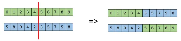
One Point Crossover
In this one-point crossover, a random crossover point is selected and the tails of its two parents are swapped to get new off-springs.
Multi Point Crossover
Multi point crossover is a generalization of the one-point crossover wherein alternating segments are swapped to get new off-springs.
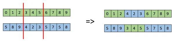
Uniform Crossover
In a uniform crossover, we don’t divide the chromosome into segments, rather we treat each gene separately. In this, we essentially flip a coin for each chromosome to decide whether or not it’ll be included in the off-spring. We can also bias the coin to one parent, to have more genetic material in the child from that parent.

Mutation
After crossover, a mutation operation is performed on the offspring. Mutation randomly changes some of the genes in the offspring's chromosome. The goal of mutation is to introduce new genetic material into the population and prevent premature convergence to a suboptimal solution.
Bit Flip Mutation
In this bit flip mutation, we select one or more random bits and flip them. This is used for binary encoded GAs.

Random Resetting
Random Resetting is an extension of the bit flip for the integer representation. In this, a random value from the set of permissible values is assigned to a randomly chosen gene.

Swap Mutation
In swap mutation, we select two positions on the chromosome at random, and interchange the values. This is common in permutation based encodings.
Inversion Mutation
In inversion mutation, we select a subset of genes like in scramble mutation, but instead of shuffling the subset, we merely invert the entire string in the subset.

These three operations are repeated for multiple generations, with the best individuals from each generation being selected for the next generation. Over time, the GA converges to an optimal solution to the optimization problem. The parameters of the GA, such as the population size, selection method, crossover rate, and mutation rate, can be adjusted to improve the performance of the algorithm for a specific problem.
GA syntax's
x = ga(fun,nvars)
x = ga(fun,nvars,A,b)
x = ga(fun,nvars,A,b,Aeq,beq)
x = ga(fun,nvars,A,b,Aeq,beq,lb,ub)
x = ga(fun,nvars,A,b,Aeq,beq,lb,ub,nonlcon)
x = ga(fun,nvars,A,b,Aeq,beq,lb,ub,nonlcon,options)
x = ga(fun,nvars,A,b,Aeq,beq,lb,ub,nonlcon,intcon)
x = ga(fun,nvars,A,b,Aeq,beq,lb,ub,nonlcon,intcon,options)
x = ga(problem)
[x,fval] = ga(___)
[x,fval,exitflag,output] = ga(___)
[x,fval,exitflag,output,population,scores] = ga(___)
Stalagmites
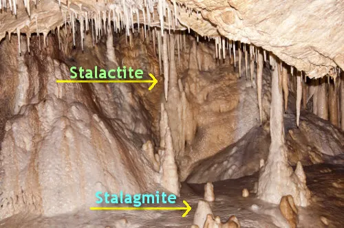
A stalagmite is a type of speleothem, which is a mineral deposit that forms in a cave or cavern. Stalagmites are formed when water drips from the ceiling of a cave and deposits minerals on the floor. As each drop of water falls, it leaves behind a tiny deposit of minerals, which can build up over time to form a cone-shaped or columnar stalagmite. Stalagmites typically form from calcium carbonate minerals, such as calcite, and can take thousands or even millions of years to grow to their full size. They are often found in caves and caverns around the world and can vary in size from just a few centimeters to several meters in height. Stalagmites are often used by scientists to study past climate and environmental changes, as the layers of mineral deposits can provide a record of changes in precipitation, temperature, and other environmental factors over time.
The following function formula we use for stalagmite in MATLAB for finding global maxima
`f(x,y) = f_(1,x) f_(2,x) f_(1,y) f_(2,y)`
`f_(1,x) = [sin(5.1pix + 0.5]^6`
`f_(1,y) = [sin(5.1piy+0.5)]^6`
`f_(2,x) = exp[-4ln(2)((x-0.0667)^2/0.64)]`
`f_(2,y) = exp[-4ln(2)((y-0.0667)^2/0.64)]`
MATLAB code for Genetic Algorithm
First we will see the function code for stalagmite.
function [f]  = stalagmite(input_vector) %defining the function for stalagmite as stalagmite(input_vector)

x = input_vector(1); %taking x = input_vector
y = input_vector(2); %taking y = input_vector

%Next formula for stalagmite function f(x,y) = f1_x f2_x f1_y f2_y

f1_x = [sin(5.1*pi*x+0.5)]^6; %Formula f1_x = [sin(5.1*pi*x+0.5)]^6
f1_y = [sin(5.1*pi*y+0.5)]^6; %Formula f1_y = [sin(5.1*pi*y+0.5)]^6

f2_x = exp(-4*log(2)*(((x-0.0667)^2)/0.64)); %Formula f2_x = exp(-4*log(2)*(((x-0.0667)^2)/0.64))
f2_y = exp(-4*log(2)*(((y-0.0667)^2)/0.64)); %Formula f2_y = exp(-4*log(2)*(((y-0.0667)^2)/0.64))

f = -(f1_x*f1_y*f2_x*f2_y); %As we know ga takes the minima value hence giving '-' to the function that inverts the result f = -(f1_x*f1_y*f2_x*f2_y)

end %End function
Step wise explanation of the code
clear all
close all
clc

%Defining our search space

x = linspace(0,0.6,150); %Taking x = linspace(0,0.6,150)
y = linspace(0,0.6,150); %Taking y = linspace(0,0.6,150)

%creating a two Dimensional mesh

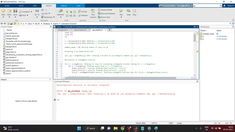
[xx, yy] = meshgrid(x,y); %For creating a 2D mesh we use meshgrid command [xx, yy] = meshgrid(x,y)

%Evaluation of stalagmite function

for i = 1:length(xx)  %Taking for loop for evaluating stalagmite function taking for i = 1:length(xx)
    for j = 1:length(yy) %Taking nested loop as j = 1:length(yy)
        input_vector(1) = xx(i,j); %Taking input_vector(1) = xx(i,j)
        input_vector(2) = yy(i,j); %Taking input_vector(2) = yy(i,j)
        f(i,j) = stalagmite(input_vector);  %calling stalagmite function here for f(i,j) = stalagmite(input_vector)

    end %ending nested loop

end %Ending main loop

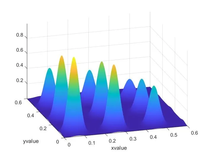
surfc(xx,yy,-f) %Contour plot under surface plot basically to visualize my function

xlabel('xvalue') %labelling x axes
ylabel('yvalue') %labelling y axes

shading interp %shading interp varies the color in each line segment and face by interpolating the colormap index or true color value across the line or face.

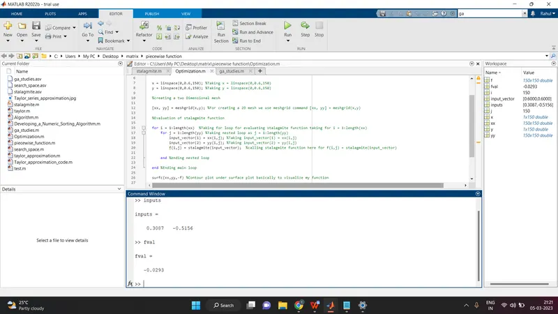
[inputs, fval] = ga(@stalagmite,2); %using ga inbuilt solver and call the stalagmite function to optimise it
Step wise explanation of the code
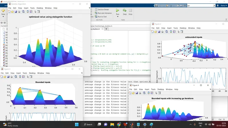
Ouput for the code
Command window
Third main code with 3 studies
clear all
close all
clc

x = linspace(0,0.6,150); %Taking x = linspace(0,0.6,150)
y = linspace(0,0.6,150); %Taking y = linspace(0,0.6,150)

number_cases = 50; %Giving number of cases as 50

%creating a two Dimensional mesh

[xx, yy] = meshgrid(x,y); %For creating a 2D mesh we use meshgrid command [xx, yy] = meshgrid(x,y)

%Evaluation of stalagmite function

for i = 1:length(xx)  %Taking for loop for evaluating stalagmite function taking for i = 1:length(xx)
    for j = 1:length(yy) %Taking nested loop as j = 1:length(yy)
        input_vector(1) = xx(i,j); %Taking input_vector(1) = xx(i,j)
        input_vector(2) = yy(i,j); %Taking input_vector(2) = yy(i,j)
        f(i,j) = stalagmite(input_vector);  %calling stalagmite function here for f(i,j) = stalagmite(input_vector)

    end %ending nested loop

end %Ending main loop

%Figure 1 for showing the optimized value using stalagmite function

options = optimoptions('ga','plotFcn',@gaplotbestf,'PopulationSize',200); %Create optimization options options = optimoptions(SolverName,Name,Value)
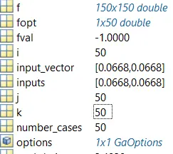
[input_vector,fval] = ga(@stalagmite,2,[],[],[],[],[0;0],[1;1],[],options); % Taking this formula x = ga(fun,nvars,A,b,Aeq,beq,lb,ub,nonlcon,options)

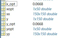
x_opt = input_vector(1); %Giving x_opt = input_vector(1)
y_opt = input_vector(2); %Giving y_opt = input_vector(2)
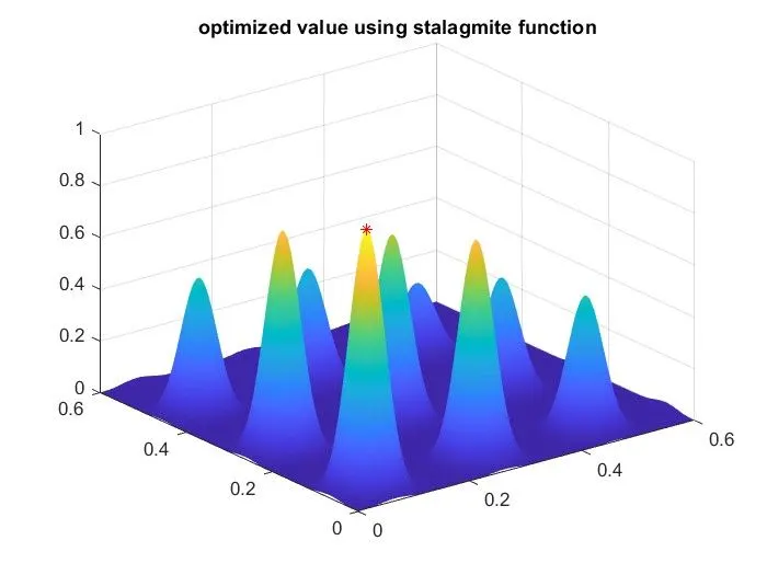
figure(1)
surf(xx, yy, -f);%Contour plot under surface plot basically to visualize my function
shading interp  %shading interp varies the color in each line segment and face by interpolating the colormap index or true color value across the line or face.
hold on %hold on
plot3(x_opt,y_opt,-fval,'r*','MarkerSize',5) %plotting plot3(x_opt,y_opt,-fval,'r*','MarkerSize',5)
title('optimized value using stalagmite function') %giving title ('optimized value using stalagmite function')

%Performing study 1 - statistical behaviour

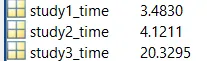
tic %Timer to know how long the matlab takes to solve the program

for i = 1:number_cases %For loop i = 1:number_cases
    [inputs, fopt(i)] = ga(@stalagmite,2); %calling function with ga solver [inputs, fopt(i)] = ga(@stalagmite,2)
    xopt(i) = inputs(1); %Taking  xopt(i) = inputs(1)
    yopt(i) = inputs(2); %Taking yopt(i) = inputs(2)

end %Ending the loop
study1_time = toc; %Stop timer

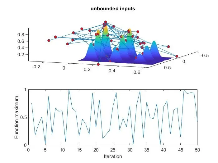
figure(2) %Figure 2
subplot(2,1,1) %Create axes in tiled positions subplot(2,1,1)
hold on %hold on
surfc(x, y, -f) %Contour plot under surface plot basically to visualize my function
shading interp %shading interp varies the color in each line segment and face by interpolating the colormap index or true color value across the line or face.
plot3(xopt,yopt,-fopt,'marker','o','markerSize',5,'markerfaceColor','r') %Plotting plot3(xopt,yopt,-fopt,'marker','o','markerSize',5,'markerfaceColor','r')
title('unbounded inputs') %Giving title title('unbounded inputs')
subplot(2,1,2) %subplot(2,1,2) Create axes in tiled positions
plot(-fopt) %plot(-fopt)
xlabel('Iteration') %labelling x axes
ylabel('Function maximum') %labelling y axes


% Performing study 2 - statistical behaviour - (with upper and lower bounds)

tic %Timer to know how long the matlab takes to solve the program
for j = 1:number_cases %for j = 1:number_cases
    [inputs,fopt(j)] = ga(@stalagmite,2,[],[],[],[],[0;0],[1;1]); %%calling function with ga solver [inputs,fopt(j)] = ga(@stalagmite,2,[],[],[],[],[0;0],[1;1])
    xopt(j) = inputs(1); %Taking xopt(j) = inputs(1)
    yopt(j) = inputs(2); %Taking yopt(j) = inputs(2)

end %Ending the loop

study2_time = toc; %Stop timer

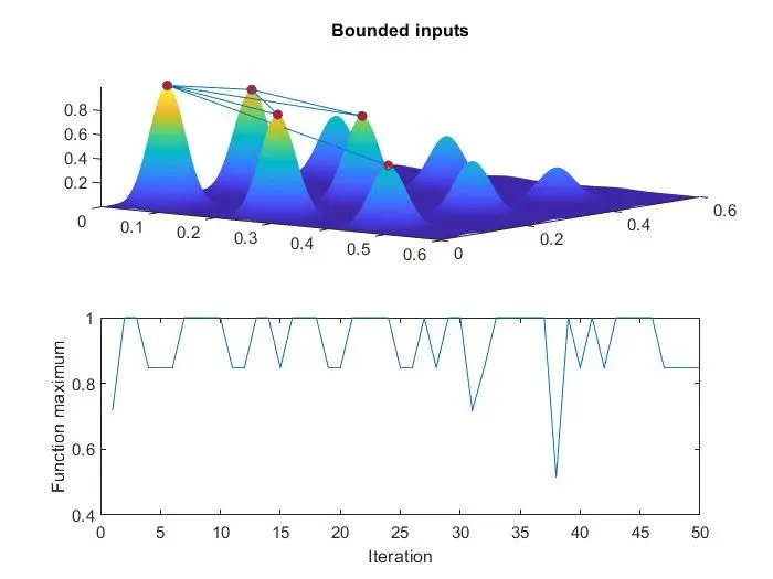
figure(3) %Figure 3
subplot(2,1,1) %Create axes in tiled positions subplot(2,1,1)
hold on %hold on
surfc(x, y, -f) %Contour plot under surface plot basically to visualize my function
shading interp %shading interp varies the color in each line segment and face by interpolating the colormap index or true color value across the line or face.
plot3(xopt,yopt,-fopt,'marker','o','markerSize',5,'markerfaceColor','r') %plotting plot3(xopt,yopt,-fopt,'marker','o','markerSize',5,'markerfaceColor','r')
title('Bounded inputs') %Giving title ('Bounded inputs')
subplot(2,1,2) %subplot(2,1,2) Create axes in tiled positions
plot(-fopt) %plotting plot(-fopt)
xlabel('Iteration') %labelling x axes
ylabel('Function maximum') %labelling y axes


%Performing study 3 - increasing GA iterations

options = optimoptions('ga');  %Taking options for optimaisation options = optimoptions('ga')
options = optimoptions(options,'PopulationSize',450); %Taking options = optimoptions(options,'PopulationSize',450)

tic %Timer to know how long the matlab takes to solve the program
for k = 1:number_cases %Taking loop for k = 1:number_cases
    [inputs,fopt(k)] = ga(@stalagmite,2,[],[],[],[],[0;0],[1;1],[],[],options); %Taking [inputs,fopt(k)] = ga(@stalagmite,2,[],[],[],[],[0;0],[1;1],[],[],options)
    xopt(k) = inputs(1); %Taking xopt(k) = inputs(1)
    yopt(k) = inputs(2); %Taking yopt(k) = inputs(2)

end %Ending the loop
study3_time = toc; %Stop timer

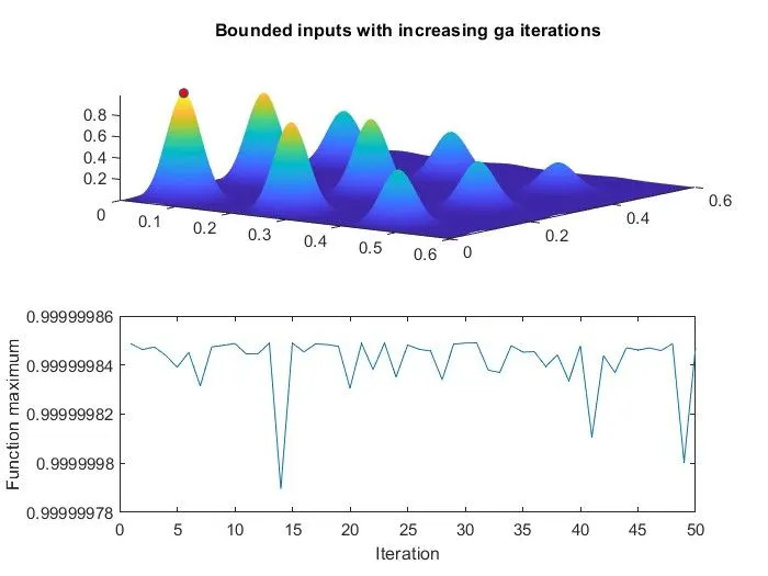
figure(4) %Figure 4
subplot(2,1,1) %Create axes in tiled positions subplot(2,1,1)
hold on %hold on
surfc(x, y, -f) %Contour plot under surface plot basically to visualize my function
shading interp %shading interp varies the color in each line segment and face by interpolating the colormap index or true color value across the line or face.
plot3(xopt,yopt,-fopt,'marker','o','markerSize',5,'markerfaceColor','r') %plotting plot3(xopt,yopt,-fopt,'marker','o','markerSize',5,'markerfaceColor','r')
title('Bounded inputs with increasing ga iterations') %Giving title('Bounded inputs with increasing ga iterations')
subplot(2,1,2) %%subplot(2,1,2) Create axes in tiled positions
plot(-fopt) %plotting plot(-fopt)
xlabel('Iteration') %labelling x axes
ylabel('Function maximum') %labelling y axes
Step wise explanation of the code