Project 1 - Parsing NASA thermodynamic data
Report for Project 1 : Parsing NASA thermodynamic data
Aim : As given NASA came up with polynomials that can be used to evaluate thermodynamic properties such as Cp, H and S. They have also documented the co-efficients that are required to evaluate these polynomials for 1000+ species. So our challenge is to create a function that extracts the 14 co-efficients and calculates the enthalpy, entropy and specific heats for all the species in the data file 'Thermo.dat'. The FIRST 7 coefficients are HIGH-temperature coefficients and the SECOND 7 coefficients are LOW-temperature coefficients. Also use the LOCAL TEMPERATURE RANGES should calculate the molecular weight of each species and should display the same in the command window generate Cp, H and S plots for all species and create sepearate folders containing this plots.
Objective : 1) Write a function that extracts the 14 co-efficients and calculates the enthalpy, entropy and specific heats for all the species in the data file. We should read the NASA Thermodynamic file called 'THERMO.dat' file. The formula to be used are:
`(Cp)/R = a1 + a2 (T) + a3 (T^2) + a4(T^3)+a5 (T^4)`
`H/(RT) = a1 + a2 (T)/2 +a3 (T^2)/3 + a4 (T^3)/4 + a5(T^4)/5 + (a6)/T`
`S/R = a1ln(T) + a2 (T) + a3(T^2) /2 + a4 (T^3)/3 + a5(T^4)/4 + a7`
Here R is the universal gas constant the value of R = 8.31446261815324 joules per kelvin (K) per mole.
2) The FIRST 7 coefficients are HIGH-temperature coefficients and the SECOND 7 coefficients are LOW-temperature coefficients. Use the LOCAL TEMPERATURE RANGES which is unique for each individual species, not the GLOBAL TEMPERATURE RANGE.
3) Calculate the molecular weight of each species and display it in the command window.
4) Plot the Cp, Enthalpy and Entropy for the local temperature range (low temperature : high temperature) specific for each species.
5) Save the plots as images with appropriate names and dump them in separate folders for each species with suitable name. All these should be generated automatically.
6) The main program that is "THERMO.dat" file should be taken as an input and generate Cp, H and S plots.
7) At the end Screenshot of the window where all the folders are saved. Plots for o2, N2 and Co2 species.
Theory part for better understanding
'THERMO.DAT' file includes.
THERMO
   300.000  1000.000  5000.000
! GRI-Mech Version 3.0 Thermodynamics released 7/30/99
! NASA Polynomial format for CHEMKIN-II
! see README file for disclaimer
O                 L 1/90O   1               G   200.000  3500.000  1000.000    1
 2.56942078E+00-8.59741137E-05 4.19484589E-08-1.00177799E-11 1.22833691E-15    2
 2.92175791E+04 4.78433864E+00 3.16826710E+00-3.27931884E-03 6.64306396E-06    3
-6.12806624E-09 2.11265971E-12 2.91222592E+04 2.05193346E+00                   4
O2                TPIS89O   2               G   200.000  3500.000  1000.000    1
 3.28253784E+00 1.48308754E-03-7.57966669E-07 2.09470555E-10-2.16717794E-14    2
-1.08845772E+03 5.45323129E+00 3.78245636E+00-2.99673416E-03 9.84730201E-06    3
-9.68129509E-09 3.24372837E-12-1.06394356E+03 3.65767573E+00                   4
H                 L 7/88H   1               G   200.000  3500.000  1000.000    1
 2.50000001E+00-2.30842973E-11 1.61561948E-14-4.73515235E-18 4.98197357E-22    2
 2.54736599E+04-4.46682914E-01 2.50000000E+00 7.05332819E-13-1.99591964E-15    3
 2.30081632E-18-9.27732332E-22 2.54736599E+04-4.46682853E-01                   4
H2                TPIS78H   2               G   200.000  3500.000  1000.000    1
 3.33727920E+00-4.94024731E-05 4.99456778E-07-1.79566394E-10 2.00255376E-14    2
-9.50158922E+02-3.20502331E+00 2.34433112E+00 7.98052075E-03-1.94781510E-05    3
 2.01572094E-08-7.37611761E-12-9.17935173E+02 6.83010238E-01                   4
OH                RUS 78O   1H   1          G   200.000  3500.000  1000.000    1
 3.09288767E+00 5.48429716E-04 1.26505228E-07-8.79461556E-11 1.17412376E-14    2
 3.85865700E+03 4.47669610E+00 3.99201543E+00-2.40131752E-03 4.61793841E-06    3
-3.88113333E-09 1.36411470E-12 3.61508056E+03-1.03925458E-01                   4
H2O               L 8/89H   2O   1          G   200.000  3500.000  1000.000    1
 3.03399249E+00 2.17691804E-03-1.64072518E-07-9.70419870E-11 1.68200992E-14    2
-3.00042971E+04 4.96677010E+00 4.19864056E+00-2.03643410E-03 6.52040211E-06    3
-5.48797062E-09 1.77197817E-12-3.02937267E+04-8.49032208E-01                   4
HO2               L 5/89H   1O   2          G   200.000  3500.000  1000.000    1
 4.01721090E+00 2.23982013E-03-6.33658150E-07 1.14246370E-10-1.07908535E-14    2
 1.11856713E+02 3.78510215E+00 4.30179801E+00-4.74912051E-03 2.11582891E-05    3
-2.42763894E-08 9.29225124E-12 2.94808040E+02 3.71666245E+00                   4
H2O2              L 7/88H   2O   2          G   200.000  3500.000  1000.000    1
 4.16500285E+00 4.90831694E-03-1.90139225E-06 3.71185986E-10-2.87908305E-14    2
-1.78617877E+04 2.91615662E+00 4.27611269E+00-5.42822417E-04 1.67335701E-05    3
-2.15770813E-08 8.62454363E-12-1.77025821E+04 3.43505074E+00                   4
C                 L11/88C   1               G   200.000  3500.000  1000.000    1
 2.49266888E+00 4.79889284E-05-7.24335020E-08 3.74291029E-11-4.87277893E-15    2
 8.54512953E+04 4.80150373E+00 2.55423955E+00-3.21537724E-04 7.33792245E-07    3
-7.32234889E-10 2.66521446E-13 8.54438832E+04 4.53130848E+00                   4
CH                TPIS79C   1H   1          G   200.000  3500.000  1000.000    1
 2.87846473E+00 9.70913681E-04 1.44445655E-07-1.30687849E-10 1.76079383E-14    2
 7.10124364E+04 5.48497999E+00 3.48981665E+00 3.23835541E-04-1.68899065E-06    3
 3.16217327E-09-1.40609067E-12 7.07972934E+04 2.08401108E+00                   4
CH2               L S/93C   1H   2          G   200.000  3500.000  1000.000    1
 2.87410113E+00 3.65639292E-03-1.40894597E-06 2.60179549E-10-1.87727567E-14    2
 4.62636040E+04 6.17119324E+00 3.76267867E+00 9.68872143E-04 2.79489841E-06    3
-3.85091153E-09 1.68741719E-12 4.60040401E+04 1.56253185E+00                   4
CH2(S)            L S/93C   1H   2          G   200.000  3500.000  1000.000    1
 2.29203842E+00 4.65588637E-03-2.01191947E-06 4.17906000E-10-3.39716365E-14    2
 5.09259997E+04 8.62650169E+00 4.19860411E+00-2.36661419E-03 8.23296220E-06    3
-6.68815981E-09 1.94314737E-12 5.04968163E+04-7.69118967E-01                   4
CH3               L11/89C   1H   3          G   200.000  3500.000  1000.000    1
 2.28571772E+00 7.23990037E-03-2.98714348E-06 5.95684644E-10-4.67154394E-14    2
 1.67755843E+04 8.48007179E+00 3.67359040E+00 2.01095175E-03 5.73021856E-06    3
-6.87117425E-09 2.54385734E-12 1.64449988E+04 1.60456433E+00                   4
CH4               L 8/88C   1H   4          G   200.000  3500.000  1000.000    1
 7.48514950E-02 1.33909467E-02-5.73285809E-06 1.22292535E-09-1.01815230E-13    2
-9.46834459E+03 1.84373180E+01 5.14987613E+00-1.36709788E-02 4.91800599E-05    3
-4.84743026E-08 1.66693956E-11-1.02466476E+04-4.64130376E+00                   4
CO                TPIS79C   1O   1          G   200.000  3500.000  1000.000    1
 2.71518561E+00 2.06252743E-03-9.98825771E-07 2.30053008E-10-2.03647716E-14    2
-1.41518724E+04 7.81868772E+00 3.57953347E+00-6.10353680E-04 1.01681433E-06    3
 9.07005884E-10-9.04424499E-13-1.43440860E+04 3.50840928E+00                   4
CO2               L 7/88C   1O   2          G   200.000  3500.000  1000.000    1
 3.85746029E+00 4.41437026E-03-2.21481404E-06 5.23490188E-10-4.72084164E-14    2
-4.87591660E+04 2.27163806E+00 2.35677352E+00 8.98459677E-03-7.12356269E-06    3
 2.45919022E-09-1.43699548E-13-4.83719697E+04 9.90105222E+00                   4
HCO               L12/89H   1C   1O   1     G   200.000  3500.000  1000.000    1
 2.77217438E+00 4.95695526E-03-2.48445613E-06 5.89161778E-10-5.33508711E-14    2
 4.01191815E+03 9.79834492E+00 4.22118584E+00-3.24392532E-03 1.37799446E-05    3
-1.33144093E-08 4.33768865E-12 3.83956496E+03 3.39437243E+00                   4
CH2O              L 8/88H   2C   1O   1     G   200.000  3500.000  1000.000    1
 1.76069008E+00 9.20000082E-03-4.42258813E-06 1.00641212E-09-8.83855640E-14    2
-1.39958323E+04 1.36563230E+01 4.79372315E+00-9.90833369E-03 3.73220008E-05    3
-3.79285261E-08 1.31772652E-11-1.43089567E+04 6.02812900E-01                   4
CH2OH             GUNL93C   1H   3O   1     G   200.000  3500.000  1000.000    1
 3.69266569E+00 8.64576797E-03-3.75101120E-06 7.87234636E-10-6.48554201E-14    2
-3.24250627E+03 5.81043215E+00 3.86388918E+00 5.59672304E-03 5.93271791E-06    3
-1.04532012E-08 4.36967278E-12-3.19391367E+03 5.47302243E+00                   4
CH3O              121686C   1H   3O   1     G   300.00   3000.00   1000.000    1
 0.03770799E+02 0.07871497E-01-0.02656384E-04 0.03944431E-08-0.02112616E-12    2
 0.12783252E+03 0.02929575E+02 0.02106204E+02 0.07216595E-01 0.05338472E-04    3
-0.07377636E-07 0.02075610E-10 0.09786011E+04 0.13152177E+02                   4
CH3OH             L 8/88C   1H   4O   1     G   200.000  3500.000  1000.000    1
 1.78970791E+00 1.40938292E-02-6.36500835E-06 1.38171085E-09-1.17060220E-13    2
-2.53748747E+04 1.45023623E+01 5.71539582E+00-1.52309129E-02 6.52441155E-05    3
-7.10806889E-08 2.61352698E-11-2.56427656E+04-1.50409823E+00                   4
C2H               L 1/91C   2H   1          G   200.000  3500.000  1000.000    1
 3.16780652E+00 4.75221902E-03-1.83787077E-06 3.04190252E-10-1.77232770E-14    2
 6.71210650E+04 6.63589475E+00 2.88965733E+00 1.34099611E-02-2.84769501E-05    3
 2.94791045E-08-1.09331511E-11 6.68393932E+04 6.22296438E+00                   4
C2H2              L 1/91C   2H   2          G   200.000  3500.000  1000.000    1
 4.14756964E+00 5.96166664E-03-2.37294852E-06 4.67412171E-10-3.61235213E-14    2
 2.59359992E+04-1.23028121E+00 8.08681094E-01 2.33615629E-02-3.55171815E-05    3
 2.80152437E-08-8.50072974E-12 2.64289807E+04 1.39397051E+01                   4
C2H3              L 2/92C   2H   3          G   200.000  3500.000  1000.000    1
 3.01672400E+00 1.03302292E-02-4.68082349E-06 1.01763288E-09-8.62607041E-14    2
 3.46128739E+04 7.78732378E+00 3.21246645E+00 1.51479162E-03 2.59209412E-05    3
-3.57657847E-08 1.47150873E-11 3.48598468E+04 8.51054025E+00                   4
C2H4              L 1/91C   2H   4          G   200.000  3500.000  1000.000    1
 2.03611116E+00 1.46454151E-02-6.71077915E-06 1.47222923E-09-1.25706061E-13    2
 4.93988614E+03 1.03053693E+01 3.95920148E+00-7.57052247E-03 5.70990292E-05    3
-6.91588753E-08 2.69884373E-11 5.08977593E+03 4.09733096E+00                   4
C2H5              L12/92C   2H   5          G   200.000  3500.000  1000.000    1
 1.95465642E+00 1.73972722E-02-7.98206668E-06 1.75217689E-09-1.49641576E-13    2
 1.28575200E+04 1.34624343E+01 4.30646568E+00-4.18658892E-03 4.97142807E-05    3
-5.99126606E-08 2.30509004E-11 1.28416265E+04 4.70720924E+00                   4
C2H6              L 8/88C   2H   6          G   200.000  3500.000  1000.000    1
 1.07188150E+00 2.16852677E-02-1.00256067E-05 2.21412001E-09-1.90002890E-13    2
-1.14263932E+04 1.51156107E+01 4.29142492E+00-5.50154270E-03 5.99438288E-05    3
-7.08466285E-08 2.68685771E-11-1.15222055E+04 2.66682316E+00                   4
CH2CO             L 5/90C   2H   2O   1     G   200.000  3500.000  1000.000    1
 4.51129732E+00 9.00359745E-03-4.16939635E-06 9.23345882E-10-7.94838201E-14    2
-7.55105311E+03 6.32247205E-01 2.13583630E+00 1.81188721E-02-1.73947474E-05    3
 9.34397568E-09-2.01457615E-12-7.04291804E+03 1.22156480E+01                   4
HCCO              SRIC91H   1C   2O   1     G   300.00   4000.00   1000.000    1
 0.56282058E+01 0.40853401E-02-0.15934547E-05 0.28626052E-09-0.19407832E-13    2
 0.19327215E+05-0.39302595E+01 0.22517214E+01 0.17655021E-01-0.23729101E-04    3
 0.17275759E-07-0.50664811E-11 0.20059449E+05 0.12490417E+02                   4
HCCOH              SRI91C   2O   1H   2     G   300.000  5000.000  1000.000    1
 0.59238291E+01 0.67923600E-02-0.25658564E-05 0.44987841E-09-0.29940101E-13    2
 0.72646260E+04-0.76017742E+01 0.12423733E+01 0.31072201E-01-0.50866864E-04    3
 0.43137131E-07-0.14014594E-10 0.80316143E+04 0.13874319E+02                   4
H2CN               41687H   2C   1N   1     G   300.00   4000.000  1000.000    1
 0.52097030E+01 0.29692911E-02-0.28555891E-06-0.16355500E-09 0.30432589E-13    2
 0.27677109E+05-0.44444780E+01 0.28516610E+01 0.56952331E-02 0.10711400E-05    3
-0.16226120E-08-0.23511081E-12 0.28637820E+05 0.89927511E+01                   4
HCN               GRI/98H   1C   1N   1     G   200.000  6000.000  1000.000    1
 0.38022392E+01 0.31464228E-02-0.10632185E-05 0.16619757E-09-0.97997570E-14    2
 0.14407292E+05 0.15754601E+01 0.22589886E+01 0.10051170E-01-0.13351763E-04    3
 0.10092349E-07-0.30089028E-11 0.14712633E+05 0.89164419E+01                   4
HNO               And93 H   1N   1O   1     G   200.000  6000.000  1000.000    1
 0.29792509E+01 0.34944059E-02-0.78549778E-06 0.57479594E-10-0.19335916E-15    2
 0.11750582E+05 0.86063728E+01 0.45334916E+01-0.56696171E-02 0.18473207E-04    3
-0.17137094E-07 0.55454573E-11 0.11548297E+05 0.17498417E+01                   4
N                 L 6/88N   1               G   200.000  6000.000  1000.000    1
 0.24159429E+01 0.17489065E-03-0.11902369E-06 0.30226245E-10-0.20360982E-14    2
 0.56133773E+05 0.46496096E+01 0.25000000E+01 0.00000000E+00 0.00000000E+00    3
 0.00000000E+00 0.00000000E+00 0.56104637E+05 0.41939087E+01                   4
NNH               T07/93N   2H   1          G   200.000  6000.000  1000.000    1
 0.37667544E+01 0.28915082E-02-0.10416620E-05 0.16842594E-09-0.10091896E-13    2
 0.28650697E+05 0.44705067E+01 0.43446927E+01-0.48497072E-02 0.20059459E-04    3
-0.21726464E-07 0.79469539E-11 0.28791973E+05 0.29779410E+01                   4
N2O               L 7/88N   2O   1          G   200.000  6000.000  1000.000    1
 0.48230729E+01 0.26270251E-02-0.95850874E-06 0.16000712E-09-0.97752303E-14    2
 0.80734048E+04-0.22017207E+01 0.22571502E+01 0.11304728E-01-0.13671319E-04    3
 0.96819806E-08-0.29307182E-11 0.87417744E+04 0.10757992E+02                   4
NH                And94 N   1H   1          G   200.000  6000.000  1000.000    1
 0.27836928E+01 0.13298430E-02-0.42478047E-06 0.78348501E-10-0.55044470E-14    2
 0.42120848E+05 0.57407799E+01 0.34929085E+01 0.31179198E-03-0.14890484E-05    3
 0.24816442E-08-0.10356967E-11 0.41880629E+05 0.18483278E+01                   4
NH2               And89 N   1H   2          G   200.000  6000.000  1000.000    1
 0.28347421E+01 0.32073082E-02-0.93390804E-06 0.13702953E-09-0.79206144E-14    2
 0.22171957E+05 0.65204163E+01 0.42040029E+01-0.21061385E-02 0.71068348E-05    3
-0.56115197E-08 0.16440717E-11 0.21885910E+05-0.14184248E+00                   4
NH3               J 6/77N   1H   3          G   200.000  6000.000  1000.000    1
 0.26344521E+01 0.56662560E-02-0.17278676E-05 0.23867161E-09-0.12578786E-13    2
-0.65446958E+04 0.65662928E+01 0.42860274E+01-0.46605230E-02 0.21718513E-04    3
-0.22808887E-07 0.82638046E-11-0.67417285E+04-0.62537277E+00                   4
NO                RUS 78N   1O   1          G   200.000  6000.000  1000.000    1
 0.32606056E+01 0.11911043E-02-0.42917048E-06 0.69457669E-10-0.40336099E-14    2
 0.99209746E+04 0.63693027E+01 0.42184763E+01-0.46389760E-02 0.11041022E-04    3
-0.93361354E-08 0.28035770E-11 0.98446230E+04 0.22808464E+01                   4
NO2               L 7/88N   1O   2          G   200.000  6000.000  1000.000    1
 0.48847542E+01 0.21723956E-02-0.82806906E-06 0.15747510E-09-0.10510895E-13    2
 0.23164983E+04-0.11741695E+00 0.39440312E+01-0.15854290E-02 0.16657812E-04    3
-0.20475426E-07 0.78350564E-11 0.28966179E+04 0.63119917E+01                   4
HCNO              BDEA94H   1N   1C   1O   1G   300.000  5000.000  1382.000    1
 6.59860456E+00 3.02778626E-03-1.07704346E-06 1.71666528E-10-1.01439391E-14    2
 1.79661339E+04-1.03306599E+01 2.64727989E+00 1.27505342E-02-1.04794236E-05    3
 4.41432836E-09-7.57521466E-13 1.92990252E+04 1.07332972E+01                   4
HOCN              BDEA94H   1N   1C   1O   1G   300.000  5000.000  1368.000    1
 5.89784885E+00 3.16789393E-03-1.11801064E-06 1.77243144E-10-1.04339177E-14    2
-3.70653331E+03-6.18167825E+00 3.78604952E+00 6.88667922E-03-3.21487864E-06    3
 5.17195767E-10 1.19360788E-14-2.82698400E+03 5.63292162E+00                   4
HNCO              BDEA94H   1N   1C   1O   1G   300.000  5000.000  1478.000    1
 6.22395134E+00 3.17864004E-03-1.09378755E-06 1.70735163E-10-9.95021955E-15    2
-1.66599344E+04-8.38224741E+00 3.63096317E+00 7.30282357E-03-2.28050003E-06    3
-6.61271298E-10 3.62235752E-13-1.55873636E+04 6.19457727E+00                   4
NCO               EA 93 N   1C   1O   1     G   200.000  6000.000  1000.000    1
 0.51521845E+01 0.23051761E-02-0.88033153E-06 0.14789098E-09-0.90977996E-14    2
 0.14004123E+05-0.25442660E+01 0.28269308E+01 0.88051688E-02-0.83866134E-05    3
 0.48016964E-08-0.13313595E-11 0.14682477E+05 0.95504646E+01                   4
CN                HBH92 C   1N   1          G   200.000  6000.000  1000.000    1
 0.37459805E+01 0.43450775E-04 0.29705984E-06-0.68651806E-10 0.44134173E-14    2
 0.51536188E+05 0.27867601E+01 0.36129351E+01-0.95551327E-03 0.21442977E-05    3
-0.31516323E-09-0.46430356E-12 0.51708340E+05 0.39804995E+01                   4
HCNN              SRI/94C   1N   2H   1     G   300.000  5000.000  1000.000    1
 0.58946362E+01 0.39895959E-02-0.15982380E-05 0.29249395E-09-0.20094686E-13    2
 0.53452941E+05-0.51030502E+01 0.25243194E+01 0.15960619E-01-0.18816354E-04    3
 0.12125540E-07-0.32357378E-11 0.54261984E+05 0.11675870E+02                   4
N2                121286N   2               G   300.000  5000.000  1000.000    1
 0.02926640E+02 0.14879768E-02-0.05684760E-05 0.10097038E-09-0.06753351E-13    2
-0.09227977E+04 0.05980528E+02 0.03298677E+02 0.14082404E-02-0.03963222E-04    3
 0.05641515E-07-0.02444854E-10-0.10208999E+04 0.03950372E+02                   4
AR                120186AR  1               G   300.000  5000.000  1000.000    1
 0.02500000E+02 0.00000000E+00 0.00000000E+00 0.00000000E+00 0.00000000E+00    2
-0.07453750E+04 0.04366000E+02 0.02500000E+02 0.00000000E+00 0.00000000E+00    3
 0.00000000E+00 0.00000000E+00-0.07453750E+04 0.04366000E+02                   4
C3H8              L 4/85C   3H   8          G   300.000  5000.000  1000.000    1
 0.75341368E+01 0.18872239E-01-0.62718491E-05 0.91475649E-09-0.47838069E-13    2
-0.16467516E+05-0.17892349E+02 0.93355381E+00 0.26424579E-01 0.61059727E-05    3
-0.21977499E-07 0.95149253E-11-0.13958520E+05 0.19201691E+02                   4
C3H7              L 9/84C   3H   7          G   300.000  5000.000  1000.000    1
 0.77026987E+01 0.16044203E-01-0.52833220E-05 0.76298590E-09-0.39392284E-13    2
 0.82984336E+04-0.15480180E+02 0.10515518E+01 0.25991980E-01 0.23800540E-05    3
-0.19609569E-07 0.93732470E-11 0.10631863E+05 0.21122559E+02                   4
CH3CHO            L 8/88C   2H   4O   1     G   200.000  6000.000  1000.000    1
 0.54041108E+01 0.11723059E-01-0.42263137E-05 0.68372451E-09-0.40984863E-13    2
-0.22593122E+05-0.34807917E+01 0.47294595E+01-0.31932858E-02 0.47534921E-04    3
-0.57458611E-07 0.21931112E-10-0.21572878E+05 0.41030159E+01                   4
CH2CHO            SAND86O   1H   3C   2     G   300.000  5000.000  1000.000    1
 0.05975670E+02 0.08130591E-01-0.02743624E-04 0.04070304E-08-0.02176017E-12    2
 0.04903218E+04-0.05045251E+02 0.03409062E+02 0.10738574E-01 0.01891492E-04    3
-0.07158583E-07 0.02867385E-10 0.15214766E+04 0.09558290E+02                   4
END
What is File parsing ?
In MATLAB, file parsing refers to the process of reading data from a file and converting it into a format that can be used by the MATLAB program. This process involves extracting relevant information from the file, such as numerical data or text, and converting it into a MATLAB variable that can be manipulated within the program. We will use use fopen and fgetl which allow to read data from different types of files, such as binary files or text files. These functions can be used to read data into MATLAB arrays or structures, depending on the format of the file.
Once the data is parsed and stored in a MATLAB variable, it can be used for further analysis or processing. For example, you can use the parsed data to create plots, perform statistical analysis, or generate reports.
File parsing is a common task in data analysis and visualization, and MATLAB provides powerful tools for this purpose.
Applications of File parsing
File parsing is a widely used technique in many fields, including data science, engineering, and finance, to name a few. Here are some examples of how file parsing is used in MATLAB.
1) Data analysis: File parsing is used to read and extract data from various types of files, including CSV files, text files, and Excel files. This data can then be processed and analyzed using MATLAB's powerful numerical and statistical functions.
2) Signal processing: MATLAB is commonly used for signal processing applications, such as audio and image processing. File parsing is used to read and convert audio and image files into a format that can be processed by MATLAB.
3) Simulation: In engineering and physics, MATLAB is used for simulating complex systems. File parsing is used to read input data and parameters from files, which are then used to set up the simulation.
4) Finance: MATLAB is widely used in the finance industry for analyzing financial data. File parsing is used to read financial data from various sources, such as stock exchange feeds, and convert it into a format that can be analyzed using MATLAB's financial toolbox.
5) Machine learning: File parsing is also an important step in machine learning applications, where large datasets need to be read and processed. In MATLAB, file parsing is used to read data into arrays or tables, which can then be used for training machine learning models.
Overall, file parsing is a crucial step in many applications, where data needs to be read from files and converted into a format that can be processed by MATLAB.
What is NASA thermodynamic file?
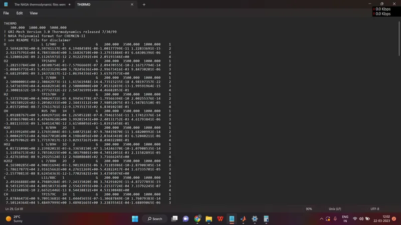
NASA thermodynamic file is a set of data files that contain thermodynamic properties of various gases and their mixtures, as well as the equations and algorithms needed to calculate those properties at various temperatures, pressures, and other conditions.
The NASA thermodynamic files were developed by the National Aeronautics and Space Administration (NASA) for use in modeling high-temperature gas flows, such as those encountered in rocket engines and re-entry vehicles. The files contain data for a wide range of gases, including hydrogen, nitrogen, oxygen, carbon dioxide, and water vapor, among others.
The thermodynamic properties provided in the NASA files include specific heat, enthalpy, entropy, and Gibbs free energy, among others. These properties are essential for predicting the behavior of gases under different conditions, such as during combustion, expansion, or compression.
The NASA thermodynamic files are widely used in the aerospace industry and are also used in other fields, such as chemical engineering and environmental science. They are implemented in software packages like CEA (Chemical Equilibrium with Applications) and NASA Glenn's Chemical Equilibrium and Applications (CEA) code, which allow researchers and engineers to simulate and analyze high-temperature gas flows and combustion processes.
What is Enthalpy (H), Entropy (S) and Specific heat (Cp)?
Enthalpy, entropy, and Cp are important thermodynamic properties that are used to describe the behavior of materials, such as gases and liquids, under various conditions.
1) Enthalpy (H): Enthalpy is a measure of the internal energy of a system, plus the work done by the system on its surroundings. It is denoted by the symbol "H" and is measured in units of energy per unit of mass (e.g. joules per kilogram). Enthalpy is a state function, meaning that it depends only on the initial and final states of the system and not on the path taken between them. In chemical reactions, enthalpy change is used to calculate the amount of heat released or absorbed during the reaction.
2) Entropy (S): Entropy is a measure of the degree of disorder or randomness in a system. It is denoted by the symbol "S" and is measured in units of energy per unit of temperature (e.g. joules per kelvin). Entropy is also a state function and is used to predict the direction of spontaneous processes. In general, the entropy of a system increases with temperature and with the degree of disorder.
3) Specific Heat Capacity (Cp): Specific heat capacity is a measure of the amount of heat required to raise the temperature of a substance by a certain amount. It is denoted by the symbol "Cp" and is measured in units of energy per unit of mass per unit of temperature (e.g. joules per kilogram per kelvin). Cp is also a state function and depends on the initial and final states of the system.
Enthalpy, entropy, and Cp are important thermodynamic properties that are used to describe the energy, disorder, and heat capacity of materials, respectively. These properties are essential for understanding the behavior of materials under various conditions, such as in chemical reactions, combustion processes, and phase transitions.
What is Universal gas constant?
The universal gas constant (also known as the molar gas constant or ideal gas constant) is a physical constant that relates the properties of a gas to its temperature, pressure, and number of moles. It is denoted by the symbol "R" and has the value of approximately 8.314 J/(mol·K) in SI units.
The universal gas constant is a fundamental constant in physics and chemistry and is used in many applications, such as in the ideal gas law, which describes the behavior of gases under different conditions. The ideal gas law states that the pressure, volume, and temperature of a gas are related by the equation.
PV = nRT
where P is the pressure, V is the volume, n is the number of moles of gas, T is the temperature, and R is the universal gas constant.
The universal gas constant is also used in other thermodynamic equations, such as the Clausius-Clapeyron equation, which relates the vapor pressure of a substance to its temperature and enthalpy of vaporization. It is also used in the Van der Waals equation, which describes the behavior of real gases, taking into account the intermolecular forces between the gas molecules.
Overall, the universal gas constant plays a fundamental role in the study of gases and is a key constant in many areas of physics and chemistry.
MATLAB code
1) The main code
clear all
close all
clc

f1 = fopen ('THERMO.dat','r'); %USing f1 as variable and fopen command for opening the file ('THERMO.dat') 'r' for read

for i = 1:5 %Creating a for loop for the first five lines using fgetl(f1)
    fgetl(f1) %fgetl (Reads the line from file, discards newline character
end  %end loop

 for i=1:53 %Again creating a for loop for all the 53 species inside which we have the main program

a = fgetl(f1); % variable a = fgetl(f1)
g = strsplit(a,' '); % using g = strsplit(a,' ') (strsplit = Split string or character vector at specified delimiter)
species = g{1};  %defining species = g{1}
LLT = str2num(g{end-3}); %For low temperature co efficients LLT = str2num(g{end-3})
LHT = str2num(g{end-2}); %For High temperature co efficients  LHT = str2num(g{end-2})
LMT = str2num(g{end-1}); % For Mid temperature co efficients  LMT = str2num(g{end-1})

line_7 = fgetl(f1); %With variable generating the co-efficients that is starting from line 7 'O' line_7 = fgetl(f1)

%first line

pos = findstr(line_7,'E'); %To know the possition of 'E' creating a variable pos = findstr(line_7,'E')

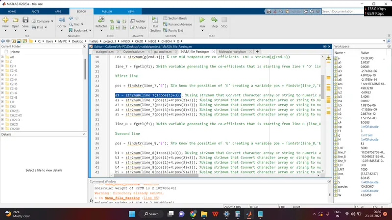
a1 = str2num(line_7(1:pos(1)+3)); %Using str2num that Convert character array or string to numeric array and inside defining position to generate first co-efficient using a1 = str2num(line_7(1:pos(1)+3))
a2 = str2num(line_7(pos(1)+4:pos(2)+3)); %Using str2num that Convert character array or string to numeric array and inside defining position to generate second co-efficient using a2 = str2num(line_7(pos(1)+4:pos(2)+3))
a3 = str2num(line_7(pos(2)+4:pos(3)+3)); %Using str2num that Convert character array or string to numeric array and inside defining position to generate Third co-efficient using a3 = str2num(line_7(pos(2)+4:pos(3)+3))
a4 = str2num(line_7(pos(3)+4:pos(4)+3)); %Using str2num that Convert character array or string to numeric array and inside defining position to generate fourth co-efficient using a4 = str2num(line_7(pos(3)+4:pos(4)+3))
a5 = str2num(line_7(pos(4)+4:pos(5)+3)); %Using str2num that Convert character array or string to numeric array and inside defining position to generate fifth co-efficient using a5 = str2num(line_7(pos(4)+4:pos(5)+3))

line_8 = fgetl(f1); %With variable generating the co-efficients that is starting from line 8 (line_8 = fgetl(f1))

%second line

pos = findstr(line_8,'E'); %To know the possition of 'E' creating a variable pos = findstr(line_8,'E')

b1 = str2num(line_8(1:pos(1)+3)); %Using str2num that Convert character array or string to numeric array and inside defining position to generate Sixth co-efficient using b1 = str2num(line_8(1:pos(1)+3))
b2 = str2num(line_8(pos(1)+4:pos(2)+3)); %Using str2num that Convert character array or string to numeric array and inside defining position to generate Seventh co-efficient using b2 = str2num(line_8(pos(1)+4:pos(2)+3))
b3 = str2num(line_8(pos(2)+4:pos(3)+3)); %Using str2num that Convert character array or string to numeric array and inside defining position to generate Eight co-efficient using b3 = str2num(line_8(pos(2)+4:pos(3)+3))
b4 = str2num(line_8(pos(3)+4:pos(4)+3)); %Using str2num that Convert character array or string to numeric array and inside defining position to generate Ninth co-efficient using b4 = str2num(line_8(pos(3)+4:pos(4)+3))
b5 = str2num(line_8(pos(4)+4:pos(5)+3)); %Using str2num that Convert character array or string to numeric array and inside defining position to generate Tenth co-efficient using b5 = str2num(line_8(pos(4)+4:pos(5)+3))

line_9 = fgetl(f1);  %With variable generating the co-efficients that is starting from line 9 (line_9 = fgetl(f1))

%Third line

pos = findstr(line_9,'E');  %To know the possition of 'E' creating a variable pos = findstr(line_9,'E')


c1 = str2num(line_9(1:pos(1)+3)); %Using str2num that Convert character array or string to numeric array and inside defining position to generate Eleventh  co-efficient using c1 = str2num(line_9(1:pos(1)+3))
c2 = str2num(line_9(pos(1)+4:pos(2)+3)); %Using str2num that Convert character array or string to numeric array and inside defining position to generate Twelveth  co-efficient using c2 = str2num(line_9(pos(1)+4:pos(2)+3))
c3 = str2num(line_9(pos(2)+4:pos(3)+3)); %Using str2num that Convert character array or string to numeric array and inside defining position to generate Thirteenth co-efficient using c3 = str2num(line_9(pos(2)+4:pos(3)+3))
c4 = str2num(line_9(pos(3)+4:pos(4)+4));  %Using str2num that Convert character array or string to numeric array and inside defining position to generate Fourteenth co-efficient using c4 = str2num(line_9(pos(3)+4:pos(4)+4))


T = linspace(LLT,LHT,400); %Using T = linspace(LLT,LHT,400) so that it creates a linear spacing between first lower temperature to the higher temperature with 400 equally spaced points
R = 8.3145; %Universal gas constant R = 8.3145

%For first 7 co-efficients

%As given the first 7 co-efficients should be Higher temperature co-efficients

if T>LMT %if else commmand if T>LMT
cp = (a1 + a2.*(T) + a3.*(T).^2 + a4.*(T).^3 + a5.*(T).^4)*R; % taking Specific heat cp formula cp = (a1 + a2.*(T) + a3.*(T).^2 + a4.*(T).^3 + a5.*(T).^4)*R;

H   = (a1.*T + (0.5*a2.*(T).^2) + ((0.33*a3.*(T).^3)) + ((0.25*a4.*(T).^4)) + ((0.2*a5.*(T).^5)) + (b1))*R; %Taking H enthalpy formula H   = (a1.*T + (0.5*a2.*(T).^2) + ((0.33*a3.*(T).^3)) + ((0.25*a4.*(T).^4)) + ((0.2*a5.*(T).^5)) + (b1))*R;

S = (a1*log(T) + a2.*(T) + ((a3.*(T).^2)./2) + ((a4.*(T).^3)./3) + ((a5.*(T).^4)./4) + b2); %Taking Entropy formula S = (a1*log(T) + a2.*(T) + ((a3.*(T).^2)./2) + ((a4.*(T).^3)./3) + ((a5.*(T).^4)./4) + b2)

%For second 7 co-efficients
%As given second 7 co-efficients should be lower temperature co-efficients

else %else
cp = (a1 + a2.*(T) + a3.*(T).^2 + a4.*(T).^3 + a5.*(T).^4)*R; %Taking specific heat cp formula cp = (a1 + a2.*(T) + a3.*(T).^2 + a4.*(T).^3 + a5.*(T).^4)*R;
H   = (a1.*T + (0.5*a2.*(T).^2) + ((a3.*(T).^3)./3) + ((a4.*(T).^4)./4) + ((a5.*(T).^5)./5) + (b1))*R; %Taking H enthalpy formula H   = (a1.*T + (0.5*a2.*(T).^2) + ((a3.*(T).^3)./3) + ((a4.*(T).^4)./4) + ((a5.*(T).^5)./5) + (b1))*R
S = (a1*log(T) + a2.*(T) + ((a3.*(T).^2)./2) + ((a4.*(T).^3)./3) + ((a5.*(T).^4)./4) + b2); %Taking S entropy formula S = (a1*log(T) + a2.*(T) + ((a3.*(T).^2)./2) + ((a4.*(T).^3)./3) + ((a5.*(T).^4)./4) + b2)
end %end if


%Combining both variables

%Plotting cp vs T, H vs T and S vs T

mkdir(species) %using mkdir() Make new folder
cd(species) %using cd() cd displays the current folder.

figure(1) %Creating sepearte figures plots figure(1) 1st figure
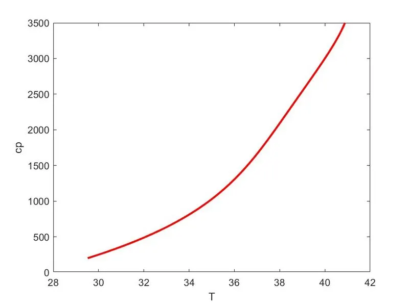
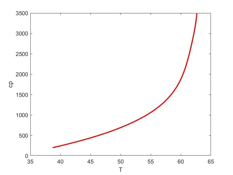
plot(cp,T,'LineWidth',2,'color','r') %using plot(), plot(cp,T,'LineWidth',2,'color','r')
xlabel('T') %labelling xlabel('T')
ylabel('cp') %labelling ylabel('cp')
title('specific heat vs Temperature') %giving a title title('specific heat vs Temperature')
saveas(figure(1),'Specific Heat vs Temperature.jpg') %saveas in folder saveas(figure(1),'Specific Heat vs Temperature.jpg')

figure(2) %Creating sepearte figures plots figure(2) 2nd figure
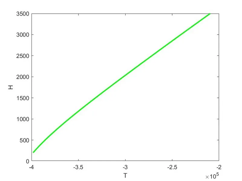
plot(H,T,'LineWidth',2,'color','g') %using plot(), plot(H,T,'LineWidth',2,'color','g')
xlabel('T') %labelling xlabel('T')
ylabel('H') %labelling ylabel('H')
title('Enthalpy vs Temperature') %giving a title title('Enthalpy vs Temperature')
saveas(figure(2),'Enthalpy vs Temperature.jpg') %saveas in folder saveas(figure(2),'Enthalpy vs Temperature.jpg')

figure(3) %Creating sepearte figures plots figure(3) 3rd figure
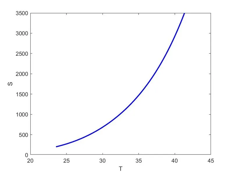
plot(S,T,'LineWidth',2,'color','b') %using plot(), plot(S,T,'LineWidth',2,'color','b')
xlabel('T') %labelling xlabel('T')
ylabel('S') %labelling ylabel('S')
title('Entropy vs Temperature') %giving a title title('Entropy vs Temperature')
saveas(figure(3),'Entropy vs Temperature.jpg') %saveas in folder saveas(figure(3),'Entropy vs Temperature.jpg')

cd .. %using cd cd displays the current folder.
W = Molecular_weight(species); % calling the function that have been created W = Molecular_weight(species);
fprintf('molecular weight of %s is %d \n',species,W); %fprintf formats data and displays the results on the screen using fprintf('molecular weight of %s is %d \n',species,W)


 end %End the loop and this repeats untill the end of species
Explanation of the main code
function [Mole_weight] = Molecular_weight(species_name) %starting function file function [Mole_weight] = Molecular_weight(species_name)
weight = 0; %defining weight = 0
elements = ['H','C','N','O','A']; %main elements are ['H','C','N','O','A']
mass = [1.008,12.011,007,15.999,39.948]; %Defining mass for each element mass = [1.008,12.011,007,15.999,39.948];
for i = 1:length(species_name) %creating a for loop inside function for i = 1:length(species_name)
    for j = 1:length(elements) %Nested for loop for j = 1:length(elements)
        if strcmpi(species_name(i),elements(j)) %giving if strcmpi(species_name(i),elements(j)) (Compare strings)
            weight = weight+mass(j); %Giving  weight = weight+mass(j)
            y = j; %variable  y = j

        end %end if
    end %end the nested loop

    number = str2double(species_name(i)); %USing  number = str2double(species_name(i)); [str2double(str) converts the text in string str to a double-precision value]
    if (number>1) %if (number>1)
        weight = weight+(mass(y)*(number-1)); %giving weight = weight+(mass(y)*(number-1))
    end %Ending if
    Mole_weight = weight; %Mole_weight = weight;

end %End main loop
end %End the function
Explanation of the code
[Defining the function file Molecular_weight]
function [Mole_weight] = Molecular_weight(species_name) %starting function file function [Mole_weight] = Molecular_weight(species_name)
`(Cp)/R = a1 + a2 (T) + a3 (T^2) + a4(T^3)+a5 (T^4)`
`H/(RT) = a1 + a2 (T)/2 +a3 (T^2)/3 + a4 (T^3)/4 + a5(T^4)/5 + (a6)/T`
`S/R = a1ln(T) + a2 (T) + a3(T^2) /2 + a4 (T^3)/3 + a5(T^4)/4 + a7`
The same step is repeated for the next second 7 set of co-efficients where we have to use Lower temperature co-efficients thus we use else here the program automatically takes mid temperature as reference and defines for lower temperature co-efficient.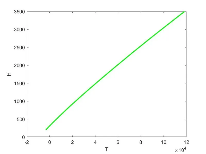
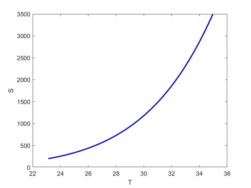
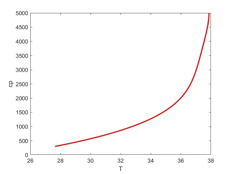
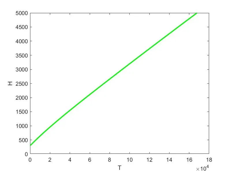
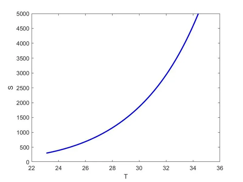
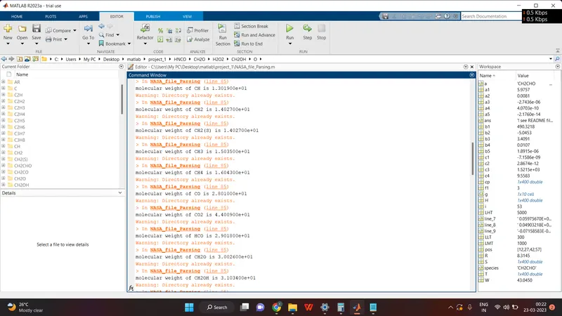
molecular weight of O is 1.599900e+01
molecular weight of O2 is 3.199800e+01
molecular weight of H is 1.008000e+00
molecular weight of H2 is 2.016000e+00
molecular weight of OH is 1.700700e+01
molecular weight of H2O is 1.801500e+01
molecular weight of HO2 is 3.300600e+01
molecular weight of H2O2 is 3.401400e+01
molecular weight of C is 1.201100e+01
molecular weight of CH is 1.301900e+01
molecular weight of CH2 is 1.402700e+01
molecular weight of CH2(S) is 1.402700e+01
molecular weight of CH3 is 1.503500e+01
molecular weight of CH4 is 1.604300e+01
molecular weight of CO is 2.801000e+01
molecular weight of CO2 is 4.400900e+01
molecular weight of HCO is 2.901800e+01
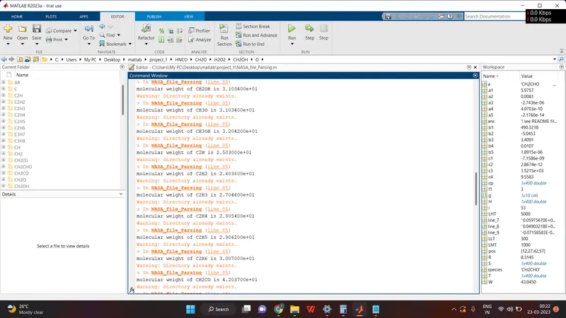
molecular weight of CH2O is 3.002600e+01
molecular weight of CH2OH is 3.103400e+01
molecular weight of CH3O is 3.103400e+01
molecular weight of CH3OH is 3.204200e+01
molecular weight of C2H is 2.503000e+01
molecular weight of C2H2 is 2.603800e+01
molecular weight of C2H3 is 2.704600e+01
molecular weight of C2H4 is 2.805400e+01
molecular weight of C2H5 is 2.906200e+01
molecular weight of C2H6 is 3.007000e+01
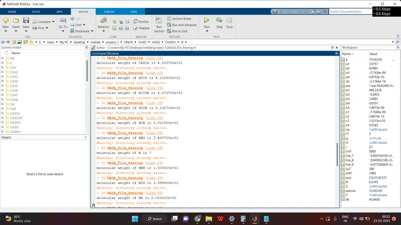
molecular weight of CH2CO is 4.203700e+01
molecular weight of HCCO is 4.102900e+01
molecular weight of HCCOH is 4.203700e+01
molecular weight of H2CN is 2.102700e+01
molecular weight of HCN is 2.001900e+01
molecular weight of HNO is 2.400700e+01
molecular weight of N is 7
molecular weight of NNH is 1.500800e+01
molecular weight of N2O is 2.999900e+01
molecular weight of NH is 8.008000e+00
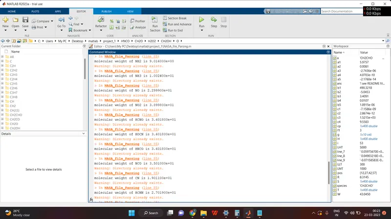
molecular weight of NH2 is 9.016000e+00
molecular weight of NH3 is 1.002400e+01
molecular weight of NO is 2.299900e+01
molecular weight of NO2 is 3.899800e+01
molecular weight of HCNO is 3.601800e+01
molecular weight of HOCN is 3.601800e+01
molecular weight of HNCO is 3.601800e+01
molecular weight of NCO is 3.501000e+01
molecular weight of CN is 1.901100e+01
molecular weight of HCNN is 2.701900e+01
molecular weight of N2 is 14
molecular weight of AR is 3.994800e+01
molecular weight of C3H8 is 4.409700e+01
molecular weight of C3H7 is 4.308900e+01
molecular weight of CH3CHO is 4.405300e+01
molecular weight of CH2CHO is 4.304500e+01
Snapshots of the command window for molecular weight
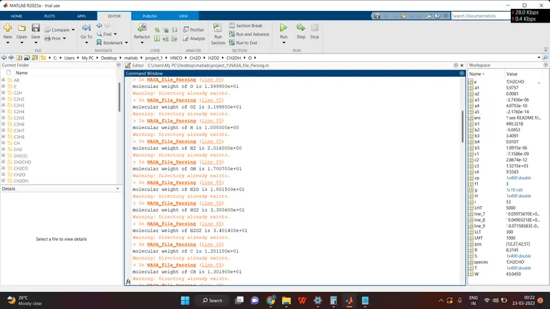
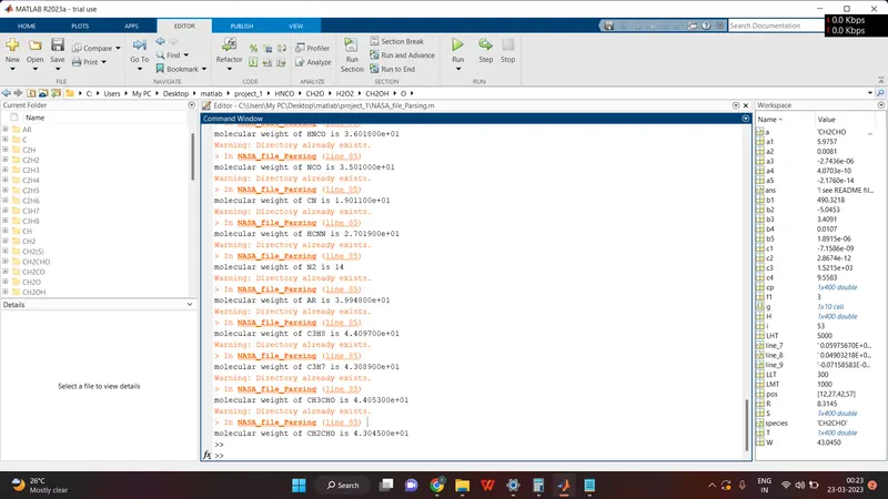
Snapshot of the file location of the folders created

Error faced while coding
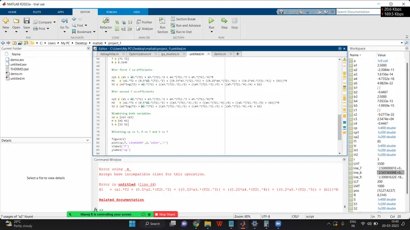
I was getting this error called Error using + "Arrays having incompatible sizes for this operations.
After that I figured where the error is in line number 24 instead of +3 I have written as +4
The corrected snapshot.