Week 4.1 - Solving second order ODEs
Report for Solving second order ODE using MatLab codes for the motion of a simple pendulum with damping
Aim: To use the MatLab code for solving second order ODE for a given expression `(d^2θ)/(dt^2) + b/m (dθ)/dt +g/L sinθ = 0` which represents the equation of motion of a simple pendulum with damping.
Objective:
1) The main objective is to solve the second order ODE for the equation `(d^2θ)/(dt^2) + b/m (dθ)/dt +g/L sinθ = 0` This equation represents the equation of motion of a simple pendulum with damping.
2) To use an ODE solver (ODE45) and use calling a function ODE for achieving our objective.
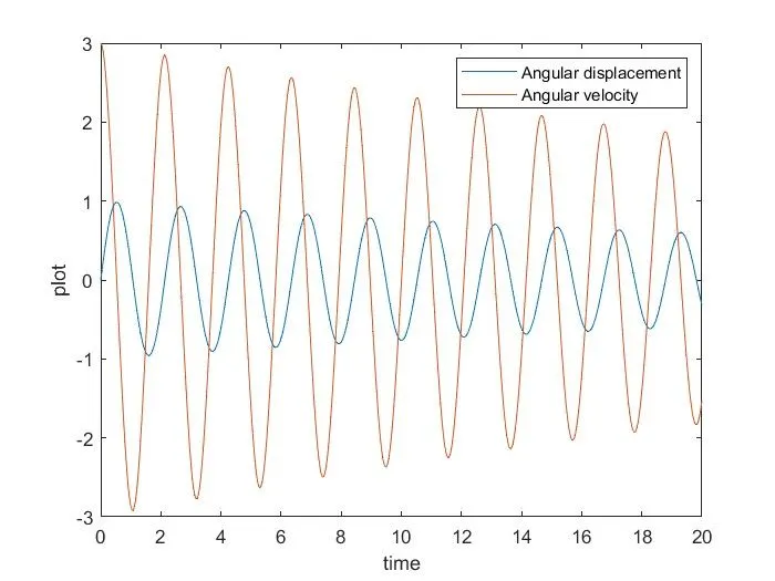
3) To Plot a figure for showing the motion of a pendulum two different waves oscillatory motion, Angular displacement and Angular velocity.
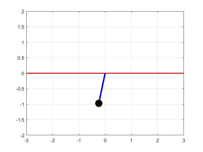
4) To animate the result and show the motion of a simple pendulum with damping with MATlab video file.
Theory part for better understanding
What is a simple pendulum?
> Pendulum a body suspended from a fixed point so that it can swing back and forth under the influence of gravity. Pendulums are used to regulate the movement of clocks because the interval of time for each complete oscillation, called the period, is constant.
The formula for the period T of a pendulum is `T = 2pi sqrt (L/g)`
where L is the length of the pendulum and g is the acceleration due to gravity.
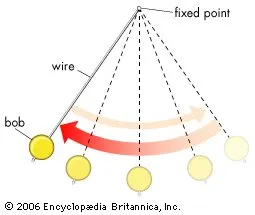
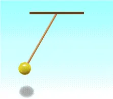
The above references show an idea of a simple pendulum and its oscillatory motion to and fro when a force is applied
The pendulum consists 3 parts
a) Fixed point or Rigid support
b) A wire or a string
C) A bob
The fixed point or rigid support holds the bob and the wire that makes the metal bob swing freely when the pendulum is at rest then the bob is at its mean position. Imagine that if the pendulum is pulled to one side and then released, it will begin to oscillate to and fro (back and forth) like a swing. The length of the pendulum is the distance along the thread from the point of suspension to the center of the bob. A pendulum's time period is determined by its length.
Simple harmonic motion (SHM)
Simple harmonic motion can be described as an oscillatory motion in which the acceleration of the particle at any position is directly proportional to the displacement from the mean position. It is a special case of oscillatory motion.
Difference between Periodic, Oscillation, and Simple Harmonic Motion
Periodic motion
- A motion repeats itself after an equal interval of time. For example, uniform circular motion.
- There is no equilibrium position.
- There is no restoring force.
- There is no stable equilibrium position.
Oscillation motion
- To and fro motion of a particle about a mean position is called an oscillatory motion in which a particle moves on either side of the equilibrium (or) mean position is an oscillatory motion.
- It is a kind of periodic motion bounded between two extreme points. For example, the Oscillation of a Simple Pendulum, the Spring-Mass System.
- The object will keep moving between two extreme points about a fixed point called the mean position (or) equilibrium position along any path. (the path is not a constraint).
- There will be a restoring force directed towards the equilibrium (or) mean position.
- In an oscillatory motion, the net force on the particle is zero at the mean position. The mean position is a stable equilibrium position.
Simple Harmonic Motion or SHM
- It is a special case of oscillation along with a straight line between the two extreme points (the path of SHM is a constraint).
- The path of the object needs to be a straight line.
- There will be a restoring force directed towards the equilibrium (or) mean position.
- The mean position in Simple harmonic motion is a stable equilibrium.
Damping
Damping is the restraining of vibratory motion, such as mechanical oscillations, noise, and alternating electric current by dissipation of energy.
Examples: 1) Unless a child keeps pumping a swing, its motion dies down because of damping.
2) Shock absorbers in automobiles and carpet pads are examples of damping devices.
A system may be so damped that it cannot vibrate. Critical damping just prevents vibration or is just sufficient to allow the object to return to its resting position in the shortest period of time.
Newton's laws of motion
Newton’s 1st law states that a body at rest or uniform motion will continue to be at rest or uniform motion until and unless a net external force acts on it.
Example: As shown in the below picture.

Newton’s 2nd law states that the acceleration of an object as produced by a net force is directly proportional to the magnitude of the net force, in the same direction as the net force, and inversely proportional to the object’s mass.
Example: As shown in the below picture.

Newton’s 3rd law states that there is an equal and opposite reaction for every action.
Example: As shown in the below picture.

Ordinary differential equations [ODE]
In mathematics, the term “Ordinary Differential Equations” also known as ODE is an equation that contains only one independent variable and one or more of its derivatives with respect to the variable. In other words, the ODE is represented as the relation having one independent variable x, the real dependent variable y, with some of its derivatives.
Types of ODE
The ordinary differential equation is classified into three types. They are:
- Autonomous ODE
- Linear ODE
- Non-linear ODE
Autonomous Ordinary Differential Equations
A differential equation which does not depend on the variable, say x is known as an autonomous differential equation.
Linear Ordinary Differential Equations
If differential equations can be written as the linear combinations of the derivatives of y, then they are called linear ordinary differential equations. These can be further classified into two types
- Homogeneous linear differential equations
- Non-homogeneous linear differential equations
Non-linear Ordinary Differential Equations
If the differential equations cannot be written in the form of linear combinations of the derivatives of y, then it is known as a non-linear ordinary differential equation.
Applications of ODE
ODEs has remarkable applications and it has the ability to predict the world around us. It is used in a variety of disciplines like biology, economics, physics, chemistry and engineering. It helps to predict the exponential growth and decay, population and species growth. Some of the uses of ODEs are:
- Modelling the growth of diseases
- Describes the movement of electricity
- Describes the motion of the pendulum, waves
- Used in Newton’s second law of motion and Law of cooling
First order differential equation
A first-order differential equation is defined by an equation: dy/dx =f (x,y) of two variables x and y with its function f(x,y) defined on a region in the xy-plane. It has only the first derivative dy/dx so that the equation is of the first order and no higher-order derivatives exist. The differential equation in first-order can also be written as follows
y’ = f (x,y) or
(d/dx) y = f (x,y)
Second order differential equation
A differential equation is an equation that consists of a function and its derivative. A differential equation that consists of a function and its second-order derivative is called a second order differential equation. Mathematically, it is written as y'' + p(x)y' + q(x)y = f(x). Second order differential equation is a specific type of differential equation that consists of a derivative of a function of order 2 and no other higher-order derivative of the function appears in the equation. It includes terms like y'', d2y/dx2, y''(x).
Examples of first and second order ODE's
First an example for differential equation we all know that A Differential Equation is an equation with a function and one or more of its derivatives

An equation which shows the function y and its derivative dy/dx
Order - An order is the highest derivative first order and second order
For a given equation `dy/dx + y^2 = 5x`, it has only the first derivative dy/dx
For a given equation `(d^2 y)/dx^2 + xy = sin(x)` This has a second derivative `(d^2y)/dx^2`, so it is a "second order" or "order 2"
Calculation
We will use a simple pendulum equation
`(d^2theta)/dt^2 + b/m (d theta)/dt + g/L sintheta = 0`

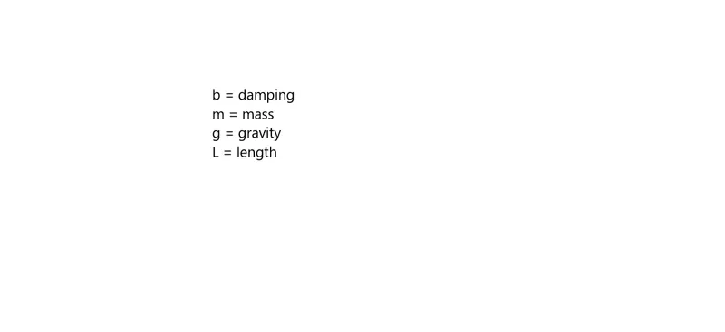
Above is a figure of a simple pendulum. Let's break it down the equation as it is in second order ODE into set of first order ODE Let's solve the equation using insert math symbol of skill lync
`theta = theta_1`
`(d theta)/dt = (d theta)/dt = theta_2` ...........eq1`
`(d theta^2)/dt^2 = (d^2theta_1)/dt^2 = d/dt ((d theta_1)/dt) = d/dt (theta_2).......eq 2`
Now,
`(d^2theta)/dt^2 + b/m (d theta)/dt + g/L sin theta = 0`
`(d^2theta_1)/dt^2 + b/m (d theta_1)/dt + g/L sin theta_1 = 0` [From eq 2 and eq 1]
`(d theta_2)/dt + b/m theta_2 + g/L sin theta_1 = 0`
Here,
First ODE
`(d theta_1)/dt = theta_2`
Second ODE
`(d theta_2)/dt = -b/m theta_2 -g/L sin theta`
This is the breaking down a second order ODE into a series of first order ODE
Now, `d/dt[[theta_1], [theta_2]] = [[theta_2],[-b/m theta_2 - g/L sin theta]]`
We will now use ODE solver now in MATlab providing in this format.
Programing of equation of motion of a simple pendulum with damping using MATlab code
clear all
close all
clc

b = 0.05;
g = 9.81;
l = 1;
m = 1;

%initial condition
theta_0 = [0,3];

%time points
t_span = linspace(0,20,500);

%ODE solver
[t,results] = ode45(@(t,theta) ode_func(t,theta, b,g,l,m), t_span, theta_0);

figure(1)
plot(t,results(:,1));
hold on
plot(t,results(:,2));
ylabel('plot')
xlabel('time')
legend('Angular displacement','Angular velocity')

value = results(:,1);
ct = 1;
for i = 1:length(value)
    total = value(i);

    figure(2)
    title('motion of a pendulum with damping')
    X0 = 0;
    Y0 = 0;
    X1 = l*cos((3*pi/2)+total);
    Y1 = l*sin((3*pi/2)+total);


    figure(2)

    plot([X0 X1],[Y0 Y1],'linewidth',3,'Color','b');
    hold on;
    plot(X1,Y1,'o','markersize',15,'markerfacecolor','k');
    hold on;
    plot([-3 3],[0 0],'lineWidth',2,'Color','r');
    hold off
    axis([-3 3 -2 2])
    grid on
    pause (0.1)
    M(ct) = getframe(gcf);
    ct = ct+1;


    M(ct) = getframe(gcf);
    ct = ct+1;

end

movie(M)
videofile = VideoWriter('motion of a Simple pendulum with damping.avi','Uncompressed AVI');
open(videofile);
writeVideo(videofile,M);
close(videofile);
ODE calling a function code
function [dtheta_dt] = ode_func(t,theta,b,g,l,m)

theta1 = theta(1)
theta2 = theta(2)
dtheta1_dt = theta2;
dtheta2_dt = -(b/m)*theta2 - (g/1)*sin(theta1);
dtheta_dt = [dtheta1_dt; dtheta2_dt];
end
Step wise explanation of the code
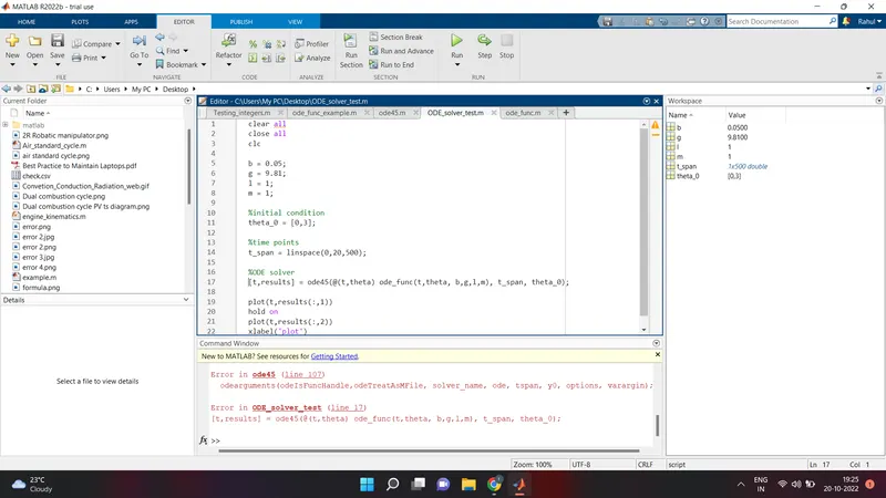
Error using odearguments
@(T,THETA)ODE_FUNC(T,THETA,B,G,L,M) returns a vector of length 1, but the length of initial
conditions vector is 2. The vector returned by @(T,THETA)ODE_FUNC(T,THETA,B,G,L,M) and the
initial conditions vector must have the same number of elements.
Error in ode45 (line 107)
odearguments(odeIsFuncHandle,odeTreatAsMFile, solver_name, ode, tspan, y0, options, varargin);
Error in ODE_solver_test (line 17)
[t,results] = ode45(@(t,theta) ode_func(t,theta, b,g,l,m), t_span, theta_0);)
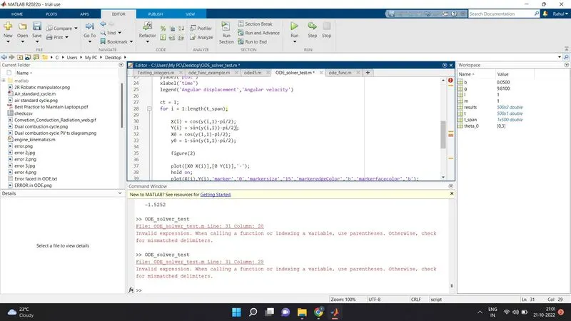
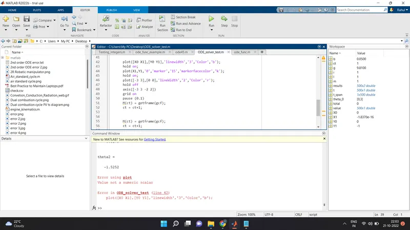
Arranged a mentor session the error was in defining function in calling function file then sorted out accordingly but again another error pops out that is error 2 below