Week 5 - Genetic Algorithm
AIM: Study about genetic algorithm and optimize the stalagmite function in matlab.
OBJECTIVE:
- Study of stalagmite function and genetic algorithm.
- Matlab code for the optimization of stalagmite function.
- Plot graph of all studies which is done over stalagmite function.
THEORY:
CONCEPT OF GENETIC ALORITHM:
Genetic algorithm is a search-based optimization technique. It works on the process of natural selection
where the fittest individual selected for the reproduction of new generation. It is used to solve both
bounded and unbounded optimization problems. It is based on natural selection theory of Charles
Darvin. For the starting purpose fix the subset of individual it means it is start with the random selection
of initial population and continuously modifying the population repeatedly creating a sequence of new
population. Now algorithm select random individuals from the current population as a parent and use it
to produce children for next generation. This successive process continue until evaluation of optimal
solution of the problem.
Genetic algorithm uses mainly three types of rules at each step for the creation of next generation.
- Selection rules: select the individuals as parent which contribute to next generation.
- Crossover rule: crossover of parent produce new children for next generation.
- Mutation rule: flip genes (make change) of parent and use for next generation.
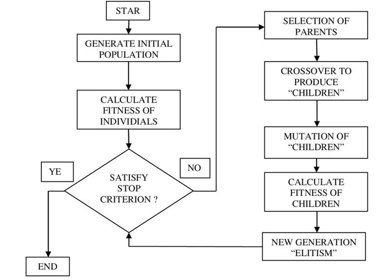
Steps in optimization of problem with genetic algorithm as-
- In step first create random initial population in starting.
- In the second step with the help of fitness values of each member calculate more fit range of
values and with the help of this it select parent for next generation. - With the help of parent and by the use of crossover rule produce children and with the help of
mutation rule make some changes in the children to create new population and replace current
population. - Algorithm stops when it reaches any of specified factors as time limit, fitness limit, constraint
limit, function tolerances etc.
FLOWCHART:
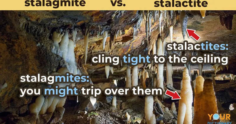
Stalagmite is basically a rock formation which arise from floor of cave due to accumulation of material
deposited from ceiling drippings. In this problem it is represented by a mathematical function called
stalagmite function. A stalagmite function has lots of local minima and local maxima. And also has one
optimal (global) maxima or minima.
SYNTAX OF ga:
In matlab syntax ‘ga’ is used for the finding of minimum of function with genetic algorithm. Syntax
explanation of ‘ga’ which is used in this study.
- x = ga(fun,nvars)
where
x= local unconstrained optimal solution
fun= objective function
nvars= number of variales
- x = ga(fun,nvars,A,b,Aeq,beq,lb,ub)
where
A,b=linear inequality constraint
Aeq,beq=linear equalities
lb,ub=lower bounds and upper bounds
If no linear equalities exist set Aeq=[] and beq=[]
- x = ga(fun,nvars,A,b,Aeq,beq,lb,ub,nonlcon,intCon,options)
where
nonlcon=nonlinear constraints
intCon=integer values
options=optimization options
If no nonlinear constraints and integer values; nonlcon and intCon are set to [].
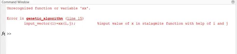
ERRORS:
Forgate to create 2D array(shows unrecognized xx variable) with help of meshgrid command it disappeared.
MATLAB CODE:
First code for stalagmite function in many scripts
%%code for stalagmite function
function A = stagalmite(input_vector)
x=input_vector(1);
y=input_vector(2);
f1=(sin(5.1*pi*x+0.5)).^6;
f2=exp((-4*log(2)*((x-0.0667).^2))/0.64);
f3=(sin(5.1*pi*y+0.5)).^6;
f4=exp((-4*log(2))*((y-0.0667).^2)/0.64);
A =-(f1*f2*f3*f4);             %negative sign invert the function plot and give maxima of function
end
Now proceed for the whole code for optimization of fuction
close all                %used to close any open window like plots and figure
clear all                %used to clear data stored in workspace
clc                      %used to clear command window

%%creation of x and y arrays and create values at 150 equal intervals
x=linspace(0,0.6,150);
y=linspace(0,0.6,150);
n=50;                    %no. of itteration

%forming 2d array by use of meshgrid with certain itteration n
[xx,yy]=meshgrid(x,y);
%%initializing i and j with the help of x and y length
for i=1:length(x)
    for j=1:length(y)
        input_vector(1)=xx(i,j);          %input value of x in stalagmite function with help of i and j
        input_vector(2)=yy(i,j);          %input value of y in stalagmite function with help of i and j
        f(i,j)=stagalmite(input_vector);  %calculate stalgmite function
    end
end
%%study 1-unbounded
tic                                %use for time calculation
for i=1:n                          %intialise i with number of itteration
    [results,fopt(i)]=ga(@stagalmite,2);  %calculating optimal values with 2 no. of variables
    xopt(i)=results(1);                   %storing optimal values of x
    yopt(i)=results(2);                   %storing optimal values of y
end
study_time1=toc                           %used to calculate time
figure(1)                                 %name as figure1
subplot(2,1,1)                            %use to plot1 which is 1 of figure1(grid 2*2)
surf(x,y,-f)                              %use for surface plot
shading interp                            %used to plot smooth plot without lines
%name of x,y axis
xlabel('x-axis');
ylabel('y-axis');
hold on                                   %used to hold plot
plot3(xopt,yopt,-fopt,'marker','o')       %use for 3D plot
subplot(2,1,2)                            %use to plot2 plot in figure1(grid 2*2)
plot(-fopt)                               %use to plot maxima of function
xlabel('no. of iteration')                %name of x axis
ylabel('function maximum')                %name of y axis

%%study 2- bounded
tic                                       %used to calculate time
for i=1:n                                 %intialise i with number of itteration
    [results,fopt(i)]=ga(@stagalmite,2,[],[],[],[],[0;0],[0.6;0.6]); %calculating optimal values with 2 no. of variables with A=[],b=[],Aeq=[],beq=[] (reason is there is no linear inequalities and linear eqalities),lb[0;0](lower limit of x and y),ub[0.6;0.6](upper limit of x and y)
    xopt(i)=results(1);                   %storing optimal values of x
    yopt(i)=results(2);                   %storing optimal values of y
end
study_time2=toc                           %used to calculate time
figure(2)                                 %name as figure2
subplot(2,1,1)                            %use to plot1 which is 1 of figure2(grid 2*2)
surf(x,y,-f)                              %use for surface plot
shading interp                            %used to plot smooth plot without lines
%name of x,y axis
xlabel('x-axis');
ylabel('y-axis');
hold on                                   %used to hold plot
plot3(xopt,yopt,-fopt,'marker','o')       %use for 3D plot
subplot(2,1,2)                            %use to plot2 plot in figure2(grid 2*2)
plot(-fopt)                               %use to plot maxima of function
xlabel('no. of iteration')                %name of x axis
ylabel('function maximum')                %name of y axis

%%study3- increased initial population
tic
options=optimoptions('ga');               %storing optimization of ga
options=optimoptions(options,'populationsize',250);         %increasing optimization size
for i=1:n                                  %intialise i with number of itteration
    [results,fopt(i)]=ga(@stagalmite,2,[],[],[],[],[0;0],[0.6;0.6],[],[],options);   %calculating optimal values with 2 no. of variables with A=[],b=[],Aeq=[],beq=[] (reason is there is no linear inequalities and linear eqalities),lb[0;0](lower limit of x and y),ub[0.6;0.6](upper limit of x and y),[],[] is no nonlinear constraint and integer value
    xopt(i)=results(1);                    %storing optimal values of x
    yopt(i)=results(2);                    %storing optimal values of y
end
study_time3=toc                            %used to calculate tim
figure(3)                                  %name as figure3
subplot(2,1,1)                             %use to plot1 which is 1 of figure3(grid 2*2)
surf(x,y,-f)                               %use for surface plot
shading interp                             %used to plot smooth plot without lines
%name of x,y axis
xlabel('x-axis');
ylabel('y-axis');
hold on                                    %used to hold plot
plot3(xopt,yopt,-fopt,'marker','o')        %use for 3D plot
subplot(2,1,2)                             %use to plot2 plot in figure3(grid 2*2)
plot(-fopt)                                %use to plot maxima of function
xlabel('no. of iteration')                 %name of x axis
ylabel('function maximum')                 %name of y axis
OUTPUTS:
Output of first study
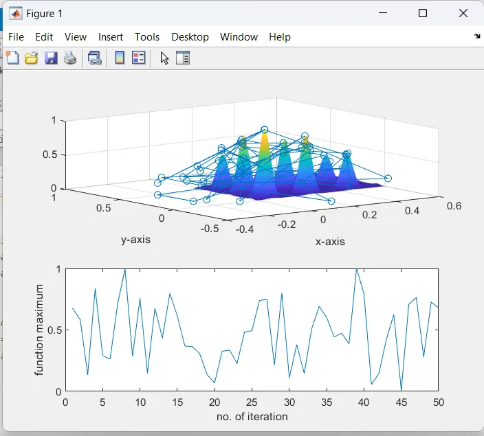
In the first study it can be obeserve that dots are appeared in large ammount. And also observed that values of x, y varies with each itteration wihch actually represent coordinate values.
Output of second study
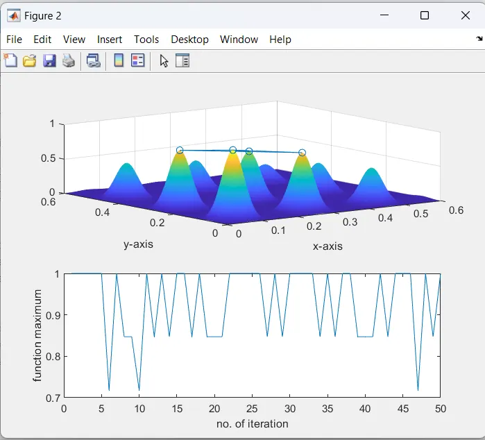
In the above plot few dots are appear in comapresion of first study. It occurs due to presence of upper and lower bounds.
Output for third study
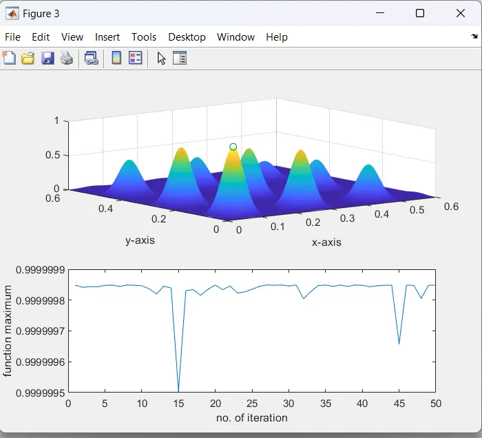
In the third study number of itterations is increased to 250 and here only one optimal point obtained which is global maxima of the function and here x=0.0668, y=0.0668 and fopt approx to 1.
REFFERENCES:
https://www.mathworks.in/help/gads/what-is-the-genetic-algorithm
https://www.tutorialspoint.com/genetic_algorithms/genetic_algorithms_introduct