Week 3.3 Air Standard Cycle

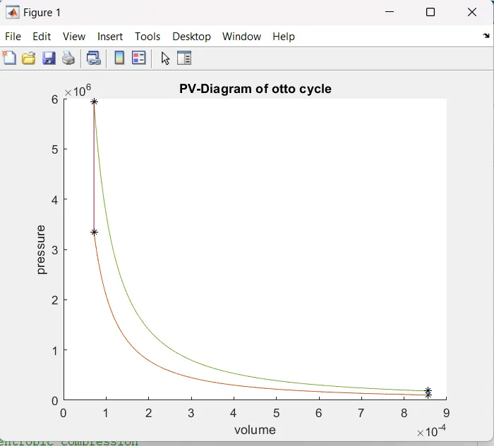
AIM: Matlab code for the air standard cycle (otto cycle) to plot PV-diagram and also calculate the thermal efficiency of the cycle.

THEORY:

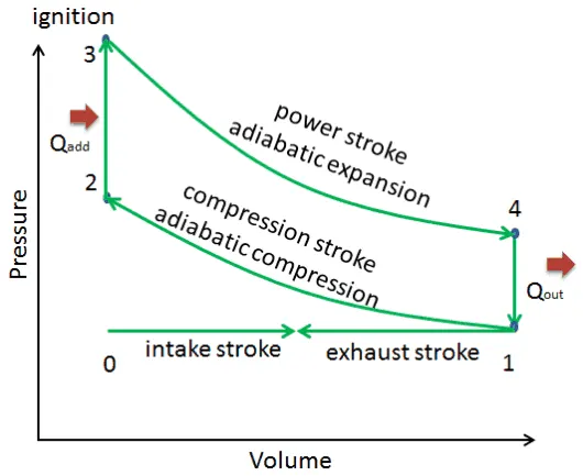
Air standard cycle use air as fuel and also consider as an ideal cycle for other cycle. Air standard cycle(otto cycle) is also a standard cycle for the spark-ignition engine. It also used to approximate the processes of petrol or diesel cycle. Actual PV-diagram is defferent from the standard cycle depend on many factors. In the otto cycle heat addition and rejection have done with constant volume and aiabatically compression and expansion occcured.

There are four processe as:

Process 1-2: Reversible adiabatic compression

Process 2-3: Constant volume heat addition process

Process 3-4: Reversible adiabatic expansion

Process 4-1: Constant volume heat rejection process

Thermal efficiency=1-(t1/t2)

Volume is change inside the engine which is traced by:

`v/v_c=1+1/2(rc-1)[R+1-cos(θ)-(R^2-sin^2(θ))^(1/2)]`

MATLAB CODE:

clear all
close all
clc

%Engine parameters are defining here
bore=0.1;
stroke =0.1;
cr=12;
cond_rod=0.15;

%Data input for the state variables
p1=103125;
t1=500;
gamma=1.4;
t3=2400;

%1-2 isentropic compression
v_swept=(pi/4)*bore^2*stroke;
v_clearnce=v_swept/(cr-1);

v1=v_swept+v_clearnce;
v2=v_clearnce;

%calculating p2 and t2 here
p2=p1*(cr)^gamma;
t2=p2*v2*t1/(p1*v1);

%calculating volume  and pressure during compression
v_compression=engine_kinematics(bore,stroke,cond_rod,cr,180,0);
c=p1*v1^gamma;
p_compression=c./(v_compression.^gamma);

%Constant volume heat addition
v3=v2;

p3=(p2*t3)/(t2);
%calculating expansion volume and pressure
v_expansion=engine_kinematics(bore,stroke,cond_rod,cr,180,360);
c=p3*v3^gamma;
p_expansion=c./(v_expansion.^gamma);

%isentropic expansion
v4=v1;
p4=p3*(v3/v4)^gamma;

%calculation of thermal efficiency
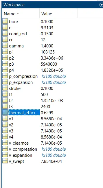
thermal_efficiency=1-(t1/t2)

figure(1)
hold on

%ploting points and joining line to make a PV diagram
plot(v1,p1,'*','color','k');
plot(v_compression,p_compression);
plot(v2,p2,'*','color','k');

plot(v3,p3,'*','color','k');
plot(v_expansion,p_expansion);
plot(v4,p4,'*','color','k');
plot([v2 v3],[p2 p3],[v4 v1],[p4 p1]);

xlabel('volume');
ylabel('pressure');
title('PV-Diagram of otto cycle');

%volume trace fomula code
function [V]=engine_kinematics(bore,stroke,cond_rod,cr,start_crank,end_crank)
a=stroke/2;
R=cond_rod/a;

v_s=pi/4*bore^2*stroke;
v_c=v_s/(cr-1);

theta=linspace(start_crank,end_crank,180);

term1=0.5*(cr-1);
term2=R+1-cosd(theta);
term3=(R^2-sind(theta).^2).^0.5;

V=(1+term1*(term2-term3)).*v_c;
end

Output:

Thermal Efficiency:

Conclusion:

PV-diagram of otto cycle is different from the actual cycle of the engine. It has curved slope for the compression and expansion is higher than actual cycle.