Curve fitting
AIM: Matlab program for curve fit.
OBJECTIVE:
- Program for linear and cubic polynomial fit.
- Plot of linear and cubic fit along with raw data points.
- Code for splitwise method.
THEORY:
Curve fitting is a method to proximate the closest values of real data. And it helps to create a curve which represent the closest proximate of real datas. It is really helpful in the establishment of functional relationship between observed dataset and parameters values etc. It is also helpful in the modeling of natural processes. Curve fit also help in the formation of function for the random increasing values.
For example: If we take population of a country there are a lot of randomness in increasing or dcreasing of population of the country. So there is no any certain formula for the prediction of population for the next year. Curve fit help to create a functional relationship for the population of country to predict values for next year. But the accuracy depend on the error in curve fit.
GOODNESS OF FIT:
For the finding of curve which satisfied almost real data points; 4 parameters to help in the finding of goodness of fit are:
- The sum of squares due to error (SSE)
- R-square
- Adjusted R-square
- Root mean squared error (RMSE)
The sum of squares due to error (SSE):
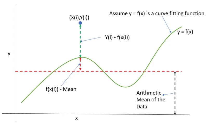
It is the sum of squares of the deviations of the data values from the predicted values(typically predicted from least squares). It helps to determine how well a independent variable fit the data.
`Err(i)=Y_i-f(x(i))`
Squaring of error and add upto the 'n' terms
`sum_(i=1)^nErr(i)^2`
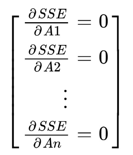
Differentiating SSE with every coefficient for finding of minima and value of coefficient by equating with 0.
R-square:
It is the square of the correlation between the response values and the predicted response values. It is also called the square of the multiple correlation coefficient and the coefficient of multiple determination. In the layman's term higher value of R-square represent better fit and lower values represent worst fit. value range between 0 to 1.
- 0 for worst fit
- 1 for better fit
Value of R-square is calculated as
`R^2=(SSR)/(SST)`
where
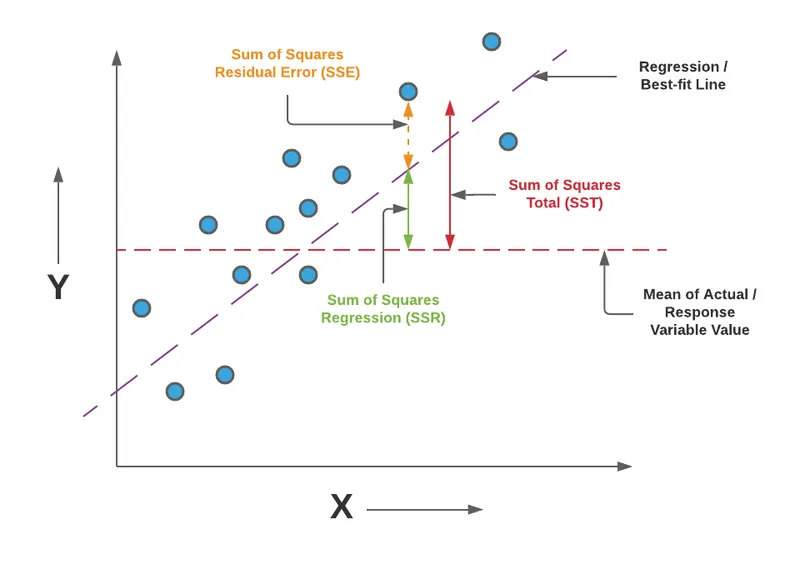
SSR = sum of square of the difference between the value of the fitting function at a given point and the arithmetic mean of the data set(regression).
if y=f(x) is the fit curve the SSR is
`SSR=sum_(i=1)^n(f(x(i))-Mean)^2`
And SSE is
`SSE=sum_(i=1)^n(Y_i-f(x(i)))^2`
Therefore SST is calculated as
SST=SSR+SSE
Adjusted R-square:
Adjusted R-square is a normalizing variation of R-square which neglects the variation of R-square due to insignificant independent variables.
- If the value of x(i) contributes to the output y, then x(i) is significant dependent variable.
- If the value of x(i) does not contributes to the output y, then x(i) is insignificant dependent variable.
adjusted R-square is calculated as:
`R_(adj)^2=1-((1-R^2)(n-1))/(n-k-1)`
where,
n= Number of datapoints
k= Number of independent variable
Root mean squared error (RMSE):
It is also known as the fit standard error and standard error of regression. It actually square root of the variance of residuals.It indicates the absolute fit of the model to the data-how close the observe data points are to the model's predicted values.
it is calculated as
`RMSE=sqrt((SSE)/n)`
where n is total no. of datapoints available.
ERROR:
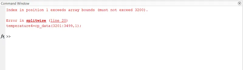
Error of exceeds array bounds or it may be say as boundary limit after insuring it within bounds which is 3200 it disappeared.
PROGRAM:
clear all
close all
clc

% Here loading data into a variable
cp_data=load('data');
temperature=cp_data(:,1);                        % Storing data for the temparatures
cp=cp_data(:,2);                % Storing the value of cp at each value of temparature

%Performing curve fit with the help of polyfit
%Use for the linear fit
co_eff1 = polyfit(temperature,cp,1);               % Using polyfit command to calculate values of a ,b
predicted_cp1 = polyval(co_eff1,temperature);      % Using polyval command to calculate the predicted values

%Use to calculate cubic fit

co_effs2 = polyfit(temperature,cp,3);               % Calculate values of the coefficents a, b, c, d
predicted_cp2 = polyval(co_effs2,temperature);      % Using polyval command to calculate the predicted values

% Compare original plot with linear curve fit
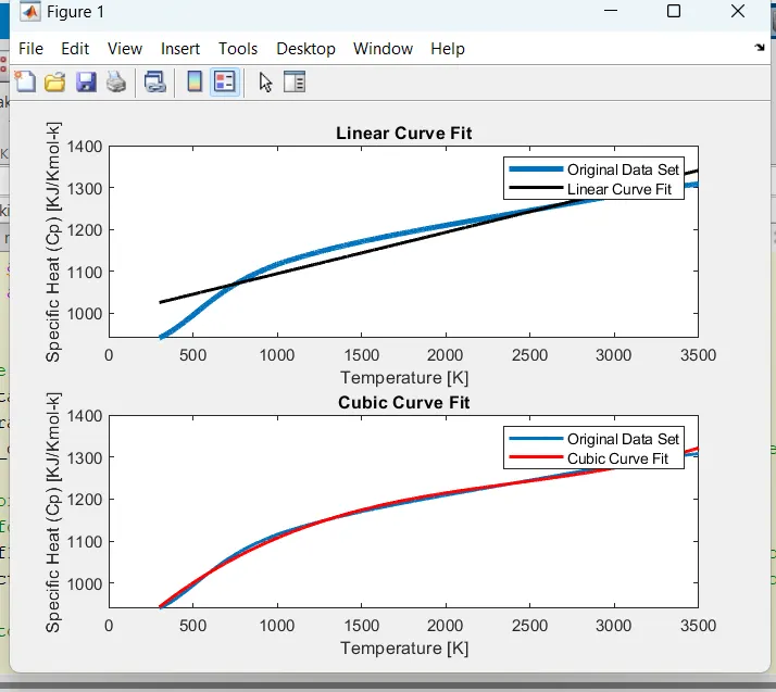
figure(1)
subplot(2,1,1)
% Use to plot original plot
plot(temperature,cp,'linewidth',3);
hold on

% Use to plot linear curve fit
plot(temperature,predicted_cp1,'linewidth',2,'color','k');
xlabel('Temperature [K]');
ylabel('Specific Heat (Cp) [KJ/Kmol-k]');
legend('Original Data Set','Linear Curve Fit');
title('Linear Curve Fit');
hold off

% Now compare the original plot with cubic curve fit

subplot(2,1,2)
% Original plot
plot(temperature,cp,'linewidth',2);
hold on

% Plotting cubic curve fit
plot(temperature,predicted_cp2,'linewidth',2,'color','r');
xlabel('Temperature [K]');
ylabel('Specific Heat (Cp) [KJ/Kmol-k]');
legend('Original Data Set','Cubic Curve Fit');
title('Cubic Curve Fit');
hold off

% Compare all plot with the help of single figure
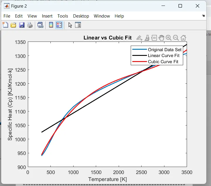
figure(2)
plot(temperature,cp,'linewidth',2);
hold on

plot(temperature,predicted_cp1,'linewidth',2,'color','k');
plot(temperature,predicted_cp2,'linewidth',2,'color','r');
xlabel('Temperature [K]');
ylabel('Specific Heat (Cp) [KJ/Kmol-k]');
legend('Original Data Set','Linear Curve Fit','Cubic Curve Fit');
title('Linear vs Cubic Fit');
hold off


% Four goodness parameters are
%   1. Sum of squares due to error (SSE)
%   2. R-square
%   3. Adjusted R-square
%   4. Root mean squared error (RMSE)

% Calculating SSE
SSE_L = sum((cp-predicted_cp1).^2);     % Use for linear curve fit
SSE_C = sum((cp-predicted_cp2).^2);     % Use for cubic curve fit

% Calculating R-square
M=mean(cp);         % Mean calculation

%% For linear curve fit
SSE_linear=sum((cp - predicted_cp1).^2);      % Sum calculation of Squared errors
SSR_linear=sum((predicted_cp1 - M).^2);       % sum calculation of squares of regression

SST_linear = SSE_linear+SSR_linear;             % Total of sum of squares

% Calculating R-square for linear curve fit
Rsquare_L = SSR_linear/SST_linear;

%% For cubic curve fit
SSE_cubic=sum((cp - predicted_cp2).^2);      % sum calculation of squared errors
SSR_cubic=sum((predicted_cp2 - M).^2);       % sum calculation of squares of regression

SST_cubic = SSE_cubic+SSR_cubic;            % Total of sum of squares

% Calculating R-square for cubic curve fit
Rsquare_C = SSR_cubic/SST_cubic;


% Here calculating all Adjusted R-square
k=1;        % Represent the number of independent variables
AdRsquare_L = 1- (((1-Rsquare_L)*(length(cp)-1))/(length(cp)-k-1));     % For linear curve fit
AdRsquare_C = 1- (((1-Rsquare_C)*(length(cp)-1))/(length(cp)-k-1));     % For cubic curve fit

% Calculate RMSE
RMSE_L = sqrt(SSE_L/length(cp));        % For linear curve fit
RMSE_C = sqrt(SSE_C/length(cp));        % For cubic curve fit

% Form a table of errors
Name_of_errors = {'SSE'; 'R_Square';'AdjustedR_Sqaure'; 'RMSE'} ;

Linear_fit_error = [SSE_L; Rsquare_L; AdRsquare_L; RMSE_L];
Cubic_fit_error = [SSE_C; Rsquare_C; AdRsquare_C; RMSE_C];

disp('Goodness Parameter for Linear and Cubic Curve fit')
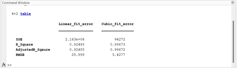
Goodness_Parameters = table(Linear_fit_error,Cubic_fit_error,'RowNames',Name_of_errors)
OUTUT:
It shows individual comparesion of curve fit and origional data.
It shows comparesion among linear,cubic curve fit to origional data curve.
Errors in the form of table
Code for splitwise method:
clear all
close all
clc

% loading all datas
cp_data = load('data');
temperature = cp_data(:,1);
cp = cp_data(:,2);

% Data split into 4 parts
temperature1=cp_data(1:1650,1);
cp1 = cp_data(1:1650,2);
% 2nd part
temperature2=cp_data(1651:2000,1);
cp2 = cp_data(1651:2000,2);
% 3rd part
temperature3=cp_data(2001:2500,1);
cp3 = cp_data(2001:2500,2);
% 4th part
temperature4=cp_data(2501:3200,1);
cp4 = cp_data(2501:3200,2);


% Considering cubic polynomial and calculating predicted value of 4 parts

co_eff1 = polyfit(temperature1,cp1,3);
pred_cp1 = polyval(co_eff1,temperature1);

co_eff2 = polyfit(temperature2,cp2,3);
pred_cp2 = polyval(co_eff2,temperature2);

co_eff3 = polyfit(temperature3,cp3,3);
pred_cp3 = polyval(co_eff3,temperature3);

co_eff4 = polyfit(temperature4,cp4,3);
pred_cp4 = polyval(co_eff4,temperature4);

% Plotting
% Original plot
plot(temperature,cp,'linewidth',6,'color','g')
hold on
% Plotting the cubic curve for the 4 regions
plot(temperature1,pred_cp1,'linewidth',2,'color','r')
plot(temperature2,pred_cp2,'linewidth',2,'color','r')
plot(temperature3,pred_cp3,'linewidth',2,'color','r')
plot(temperature4,pred_cp4,'linewidth',2,'color','r');
xlabel('Temparature (K)');
ylabel('Cp (KJ/K-mol K)');
axis([0 4000 900 1500]);
legend('Original data','Cubic Curve Fit') ;
OUTPUT:
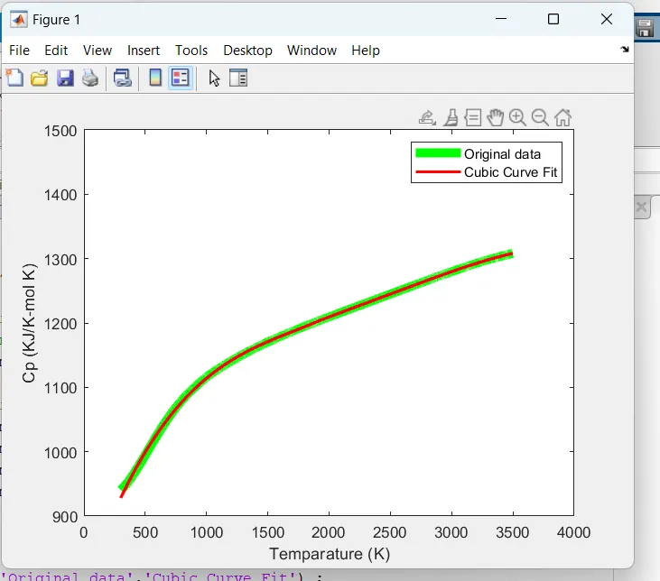
Thicker line (green) represent origional data and red line represent the curve fit of polynomial 3.
CONCLUSION:
- Linear and polynomial curve fit performed easily with the help of matlab.
- Goodness parameters help to fit the curve very accuratly with the origional data.
- Curve fit is very accurate in this case with higher value of R-square very close to 1.
REFERENCES:
https://projects.skill-lync.com/projects/Curve-Fitting-and-criterion-to-choose-best-fit-41860