Week 4.1 - Solving second order ODEs

AIM:

Matlab program for solution of second order ODE which represent equation of simple pendulum and also stimulate the pendulum motion.

THEORY:

Ordinary differential equation(ODE) is equation of one independent variable, and one or more derivatives with respect to that variable. Simple example of ODE is Newton’s second law of motion for the particle of any given mass as:

`m*(d^2x)/dt^2=f(x)`

Similarly equation of forces on spring system also result of second derivatives of the function. And pendulum movement is also depend on Newton second law is a second order of ODE.

`(d^2theta)/(dt^2)+b/m*(d(theta))/(dt)+g/L*(sintheta)=0`

g=acceleration due to gravity

L=length of string

m= mass of ball

b=damping coefficient

By the conversion of second order ODE into first order ODE to solve the pendulum differential equation.

MATLAB CODE:

%% clear command window and workspace and close other opening window
clear all
close all
clc

 %% Inputs for the operations
b=0.05;         %damping coefficient
g=9.81;         %accceleration due to gravity
l=1;            %length of line(string)
m=1;            %mass of ball(kg)

ct=1;           %variable declairation for the movie creation
               
theta_0=[0;3];  %angular velocity 

t_span=linspace(0,20,500);     %time interval

%solution of ode by the use of ode45
[t,result]=ode45(@(t,theta) ode_func(t,theta,b,g,l,m),t_span,theta_0);

%% plot the solutions of ode 
plot(t,result(:,1));
hold on
plot(t,result(:,2));
xlabel('Angular-radians');
ylabel('Angular velocity');

OUTPUT:

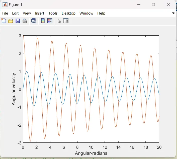
MATLAB FULL CODE:

%% clear command window and workspace and close other opening window
clear all
close all
clc

 %% Inputs for the operations
b=0.05;         %damping coefficient
g=9.81;         %accceleration due to gravity
l=1;            %length of line(string)
m=1;            %mass of ball(kg)

ct=1;           %variable declairation for the movie creation
               
theta_0=[0;3];  %angular velocity 

t_span=linspace(0,20,500);     %time interval

%solution of ode by the use of ode45
[t,result]=ode45(@(t,theta) ode_func(t,theta,b,g,l,m),t_span,theta_0);

%% plot the solutions of ode 
plot(t,result(:,1));
hold on
plot(t,result(:,2));
xlabel('Angular-radians');
ylabel('Angular velocity');

%% create and capture pendulum  
for i=1:length(result(:,1))
    %fixing the initial value of x and y
    x0=0;       
    y0=0;
    %calculating coordinates for pendulum
    x1=l*sin(result(i,1));
    y1=-l*cos(result(i,1));
    
    %creating a beam and also a line(string) for holding ball
    plot([-1,1],[0,0],'linewidth',8,'color','k');
    line([x0 x1],[y0 y1],'linewidth',2,'color','g');
    hold on
    
    %create a ball for the formation of pendulum
    plot(x1,y1,'o','markers',22,'markerfacecolor','b');
    grid on;
    %define the axis length in sequence of x and y axis
    axis([-1.5 1.5 -1.5 0.5]);
    pause(0.01);                  %time gap from one to another itteration
    hold off;
    M(ct)=getframe(gcf);          %capturing frames
    ct=ct+1;                      %increase the value of ct by 1 untill the end of loop
end

%% creation of movie and save it in avi formate 
movie(M)
videofile=VideoWriter('pendulum_animation.avi','uncompressed AVI');
open(videofile)
writeVideo(videofile,M)
close(videofile)

OUTPUT:

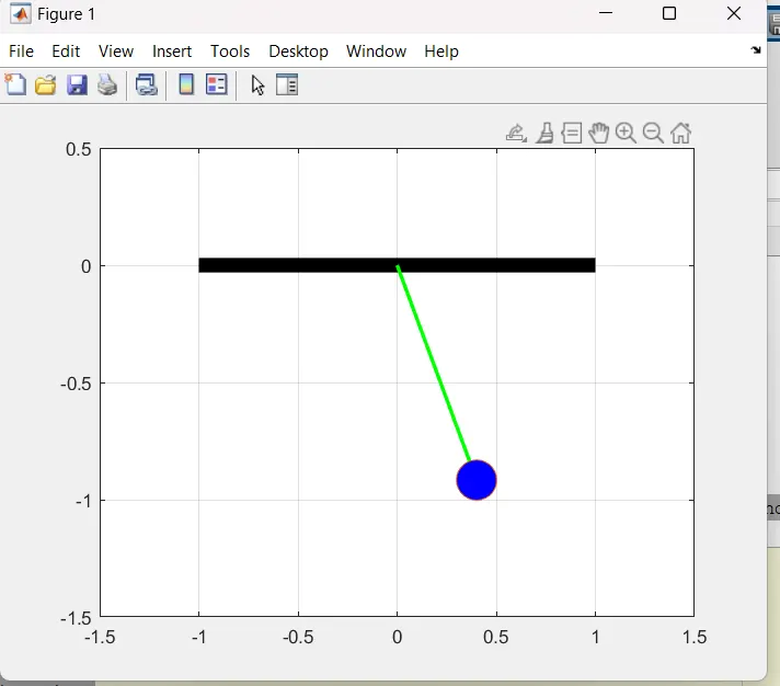
ERROR:

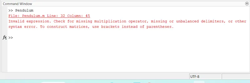
Error for the expression after write a right expression to remove the error.

LINK: https://youtu.be/JgB48EdPVVE

CONCLUSION:

The motion of pendulum mostly affected by damping coefficient so when damping coefficient increases pendulum also damped faster.