Week 5 - Genetic Algorithm

AIM: Finding the global maxima of a stalagmite function and optimizing it using MATLAB code.

OBJECTIVES:

1. Write code in MATLAB to optimize the stalagmite function and find the global maxima of the function.
2. Clearly explain the concept of genetic algorithm in your own words and also explain the syntax for ga in MATLAB in your report.
3. Make sure that your code gives the same output, even if it is made to run several times.

DESCRIPTION:

The genetic algorithm is an algorithm used for solving both constrained and unconstrained optimization problems. A genetic algorithm is a search heuristic that is inspired by Charles Darwin’s theory of natural evolution. It selects random inputs called population, check their fitness for selection, and pairing purposes (the pair is called as parents) to generate new data (called as new/next generation). This next-generation data is mutated from data acquired from parents which is essential for computing optimized output.

The genetic algorithm uses three main types of rules at each step to create the next generation from the current population:

1. Selection rules select the individuals, called parents, that contribute to the population at the next generation.
2. Crossover rules combine two parents to form children for the next generation.
3. Mutation rules apply random changes to individual parents to form children.

SYNTAX of ga:

`x=ga(fn​,ηvars​,A,b,Aeq​,beq​,lb​,Ub​)`

defines a set of lower and upper bounds on the design variables, x, so that a solution is found in the range LB ≤ x ≤ UB. (Set Aeq=[] and beq=[] if no linear equalities exist)

• The satalagmite function is defined separately. This function is later called into the main GA program.
• Now we define the x and y inputs using linspace command.
• Then the input vectors are transformed into array [xx,yy], so that it can be used to evaluate functions of two variables and plot three-dimensional mesh/surface plots.
• Now the values in the different matrixs created can be put as an input into the function that we have created,by calling it.By this we can get the value of the stalagmite function at various values of x and y.
• Now since we have got the value of the function at various values,we now need to calculate the maxima value,which can be calculated using the ga command,which is an in-built function in MATLAB.
• Then, the total number of time the ga needs to run is defined using num_cases, and with help of for loop ga is made to run for each iteration and the value is stored in an array.
• GA generally gives the minima value(in built in MATLAB), but we need the maxima hence we can just inverse the stalagmite function by introducing a 'Negative sign'(This inverses the stalagmite curve and the Global maximas can be found, instead minima)
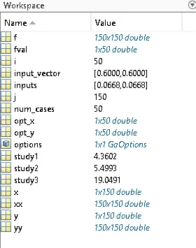
• The total study time is calculated using the 'tic' and 'toc' command at the start and end of the ga for loop respectively.
• The results are then plotted using the surfc command and plot command.
• GA is made to run for 3 iterations, with each iteration having bounded inputs , unbounded inputs and increasing population size.

GOVERNING EQUATIONS:

STALAGMITE FUNCTION:

`f ( x , y ) = f 1 , _x f _2 , _x f_ 1 ,_ y f_ 2 , y`

`f_( 1 , x) = [ sin ( 5.1 π x + 0.5 ) ] ^6`

f (1 , y) = [ sin ( 5.1 π y + 0.5 ) ] ^6`

f_( 2 , x )= exp [ − 4 ln ( 2 ) ( x − 0.0667 )^ 2/ 0.64 ]`

f _(2 , y) = exp [ − 4 ln ( 2 ) ( y − 0.0667 ) ^2 /0.64 ]`

Stalagmite function code:

function [f]= stalagmite(input_vector) % Stalagmite function with input as input_vector which contains the x and y variables.
x= input_vector(1);
y= input_vector(2);
f1= (sin(5.1*pi*x+0.5))^6;
f2= (sin(5.1*pi*y+0.5))^6;
f3= exp(-4*log(2)*(x-0.0667)^2/0.64);
f4= exp(-4*log(2)*(y-0.0667)^2/0.64);
f= -(f1*f2*f3*f4); % The Negative sign denotes the inverse of the Stalagmite function and is added in order to find the Maximum value, as GA algorithm always gives the Minimum value.
end

MAIN CODE:

clear all
close all
clc
 
% defining search space
x = linspace(0,0.6,150);
y = linspace(0,0.6,150);
% Creating a 2D mesh
[xx, yy] = meshgrid(x, y);

% Evaluating the stalagmite function
for i = 1:length(xx)
    for j = 1:length(yy)
        input_vector(1) = xx(i,j);
        input_vector(2) = yy(i,j);
        f(i,j) = stalagmite(input_vector);
    end
end

% Iteration Count
num_cases = 50;
  
% STUDY1
tic  % Study time start
for i = 1:num_cases
    [inputs, fval(i)] = ga(@stalagmite,2);
    opt_x(i) = inputs(1);
    opt_y(i) = inputs(2);
end
 study1=toc % Study time end

 % plotting unbound iteration 
figure(1)
subplot(2,1,1)
surfc(xx,yy,-f)
hold on
 
% Removing gridlines on the 3D surface plot 
shading interp
plot3(opt_x,opt_y,-fval,'marker','*','markersize',3)
title('UNBOUNDED INPUTS')
subplot(2,1,2)
plot(-fval)
xlabel('NUMBER OF ITERATIONS')
ylabel('F MAXIMUM')

% STUDY2
% BOUNDED INPUTS
tic
for i = 1:num_cases
    [inputs, fval(i)] = ga(@stalagmite,2,[],[],[],[],[0;0],[0.6;0.6]);
    opt_x(i) = inputs(1);
    opt_y(i) = inputs(2);
end
 study2=toc
 
figure(2)
subplot(2,1,1)
surfc(xx,yy,-f)
xlabel('x value')
ylabel('y value')
hold on
shading interp
plot3(opt_x,opt_y,-fval,'marker','*','markersize',3)
title('BOUNDED INPUTS')
subplot(2,1,2)
plot(-fval)
xlabel('NUMBER OF ITERATIONS')
ylabel('F MAXIMUM')

% STUDY3    
% BOUNDED INPUTS WITH ALTERED POPULATION SIZE
options = optimoptions('ga');
options = optimoptions(options,'PopulationSize',300);
tic 
for i = 1:num_cases
    [inputs, fval(i)] = ga(@stalagmite,2,[],[],[],[],[0;0],[0.6;0.6],[],[],options)
    opt_x(i) = inputs(1);
    opt_y(i) = inputs(2);
end
study3=toc

figure(3)
subplot(2,1,1)
surfc(xx,yy,-f)
xlabel('x value')
ylabel('y value')
hold on
shading interp
plot3(opt_x,opt_y,-fval,'marker','*','markersize',3)
title('BOUNDED INPUTS WITH ALTERED POPULATION SIZE')
subplot(2,1,2)
plot(-fval)
xlabel('NUMBER OF ITERATIONS')
ylabel('F MAXIMUM')

EXPLANATION:

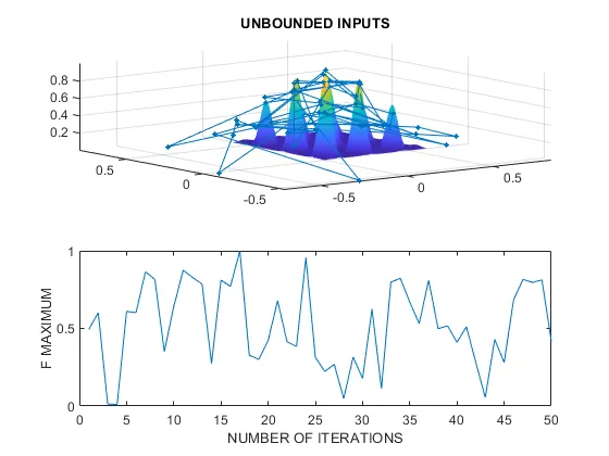
• In the first iteration, the behaviour of the algorithm is studied by not defining the limits. The GA does not run within a particular searchspace, since we have not defined bounds.
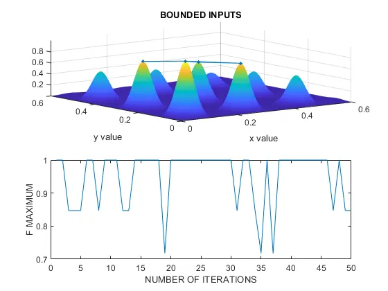
• In the second iteration,here the lower and upper bounds are defined so as to know the boundaries within which the global maxima lies. In other words we are defining a definite space within which the global maxima is to be found.
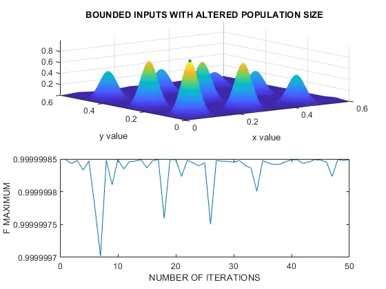
• In the last iteration, the population size is increased so as to converge to the Global maxima.

OUTPUTS:

Study1:

Study2:

Study3:

Workspace:

CONCLUSION:

By using basic commands in MatLab we got the stalagmite plot. The statistical behavior of the stalagmite plot is generated.

It can be concluded that GA gives more accurate results in case of bounded inputs and by increasing the number of iterations and population size.

It can also be infered that even if we define a particular search space for GA, the GA doesnt run inside the search space. Only in cases of bounded inputs we can get interfereable results.

REFERENCES:

https://in.mathworks.com/help/gads/what-is-the-genetic-algorithm.html

https://towardsdatascience.com/introduction-to-genetic-algorithms-including-example-code-e396e98d8bf3

https://en.wikipedia.org/wiki/Genetic_algorithm

https://in.mathworks.com/help/gads/ga.html#d120e39545