Week 3 - Solving second order ODEs

Aim:

A program to simulate the transient behaviour of a simple pendulum and to create an animation of its motion.

Objectives:

• Write a program in MATLAB to solve the given ODE using the given parameters.
• Plot the displacement & velocity w.r.t time graph.
• Create an animation of the motion of the pendulum.

Description:

A simple pendulum consists of a bob of mass 'm' suspended by string with negligible mass of length 'l'. The forces that act on the pendulum are gravitation force 'g' and the tension of the string. If the pendulum weight or bob is pulled to a relatively small angle from the vertical and let go, it will swing back and forth at a regular period and frequency. The motion of a simple pendulum is a basic classical example of simple harmonic motion,

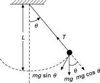
An ordinary differential equation (ODE) is a differential equation containing one or more functions of one independent variable and the derivatives of those functions.

The second order ODE equation of motion of a simple pendulum with damping:

`(d^2theta)/dt^2+b/m((d theta)/dt)+g/l(sin theta) = 0`

Where,

b = damping coefficient.

m = mass of the bob in Kg.

g = the gravity in m/s`^2`.

l = length of the string in m.

Breaking down the 2nd Order Differential Equations into two 1st Order Differential Equations,

Consider, `theta = theta_1`

Differentiating, `(d theta)/dt = (d theta_1)/dt` --------(1)

`(d theta1)/dt = theta_2`

Differentiating,

`(d^2 theta)/dt^2 = (d^2 theta_1)/dt^2 = d/dt((d theta_1)/dt) = d/dt(theta_2)` -------(2)

Substituting we get,

`(d theta_1)/dt = theta_2`

`(d theta_2)/dt = - b/m theta_2 - g/l sin theta`

From this derivation we have defined θ1 and θ2.

Inputs are taken as given in the problem:

L = 1meter

m= 1kg

b=0.05

g=9.81m/s`^2`

Algorithm:

1. First before creating the main program, create the function program to use a ode45 solver, ode_func (Anonymous function) which will return a column matrix for the solver with the reduced 1^st order equations.
2. Define the Input parameters.
3. Provide time limits and initial conditions according to the ode45 syntax
4. The results will contain two separate columns, access the result array to plot the angular velocity and angular displacement.
5. Using FOR loop capture the variation of time and plot the location of pendulum with co-ordinates varying as a function of angular displacement
6. Generate the animation using movie command.
7. Save the movie in a videofile.

MATLAB Program:

ode function:

function [dtheta_dt]=ode_func(t,theta,b,g,l,m)

theta1=theta(1)
theta2=theta(2)
dtheta1_dt=theta2;
dtheta2_dt=-(b/m)*theta2 - (g/l)*sin(theta1);
dtheta_dt=[dtheta1_dt; dtheta2_dt];

end

Main Program:

% Solving the Second order ODE of a simple pendulum and its animation

clear all 
close all
clc

% Inputs
b=0.05;    % Damping Coefficient
g=9.81;    % Gravity in m/s^2
l=1;       % Length of Pendulum in m 
m=1;       % Mass of the ball in kg

% Initial condition
theta_0=[0;3];

% Time points
t_span=linspace(0,20,500);

% Solving ODE
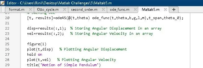
[t, results]=ode45(@(t,theta) ode_func(t,theta,b,g,l,m),t_span,theta_0);

disp=results(:,1);  % Storing Angular Displacement in an array
vel=results(:,2);   % Storing Angular Velocity in an array

figure(1)
plot(t,disp)   % Plotting Angular Displacement
hold on
plot(t,vel)   % Plotting Angular Velocity
title('Motion of Simple Pendulum')
xlabel('Time in sec')
ylabel('Amplitude')
legend('Angular Displacement(rad)','Angular Velocity(rad/s)')
grid on 
hold off

% Fixed Coordinates of one end of pendulum
x0=0;
y0=0;

ct=1; % Counter Variable

% Iteration to create the animation
for i=1:length(disp)

    % Moving coordinates of the bob
    x1 = l*sin(disp(i,1));
    y1 = -l*cos(disp(i,1));

    % Plotting the animation
    figure(2)

    % Base of the Pendulum
    plot([-1 1],[0 0],'linewidth',5,'color','k')
    hold on
    % String of the Pendulum
    plot([x0 x1],[y0 y1],'linewidth',3,'color','b')
    hold on
    % Bob of the Pendulum
    plot(x1,y1,'o','markersize',20,'markerfacecolor','r')
    title('Animation of transient behaviour of a Pendulum')
    %Axes setting
    axis([-2 2 -2 2])
    pause(0.03)
    hold off

    M(ct) = getframe(gcf);
    ct = ct+1;
end

% Converting the animation into a movie
movie(M)
videofile = VideoWriter('simple_pendulum.avi','Uncompressed AVI');
open(videofile)
writeVideo(videofile,M)
close(videofile)

Explanation:

ODE45 is usually the function of choice among the ODE solvers. It compares methods of orders four and five to estimate error and determine step size. ODE45 is so accurate that its default behavior is to use its interpolant to provide results at intermediate points.

ode_function is the function made to solve the given equation where the assumption is made in the from the code

t_span is a command used in the ode45 solver which specifies the time span of the iterations that are going to solve the ordinary differential equation.

Firstly, the given details are assigned as variables in the code. Then time span of the simple pendulum is set by using linspace command then, theta value is given as a column matrix. After this we use ode45 function and corresponding 'ode_func' function call in main program.

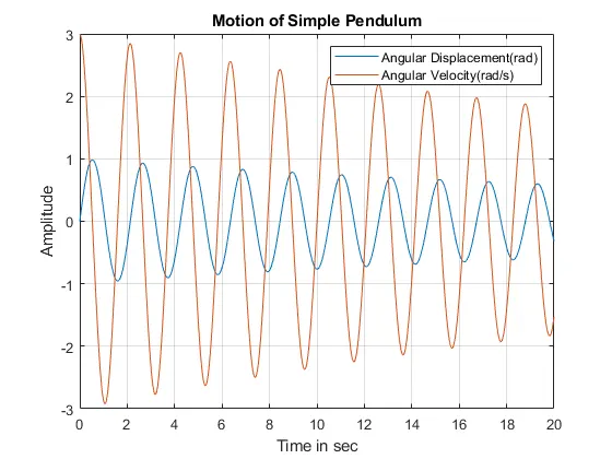
Then plot command is used to plot graph corresponding to time and velocity,legend command is used for identify each values in the graph.

For getting the accurate simulation of the simple pendulum corresponding to the second order ODE with damping we need to use the looping statements, here for loop is used to create this.

The pendulum has fixed coordinates mentioned as x0,y0 and x1, y1 are the other coordinates.

Marker command is used for making bob of the pendulum. The axis is fixed using axis command. The counter command is used to make the value changes in each for loop. Then videoWriter command is used to create the video file.

Errors:

• First Error i got while waiting for the animation to complete is not really an error. The error will go away after completing the animation. No further changes required
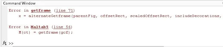
• Second Error was when i went to improvise the code from assigning the value to individual variables 'disp' and ' vel'. 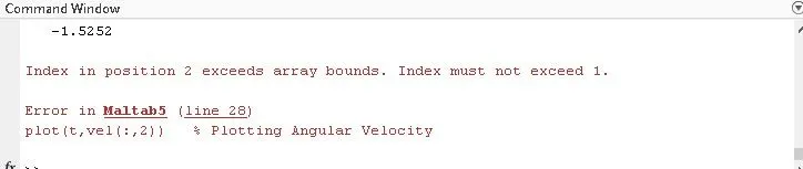But failed to change the below lines for plotting.

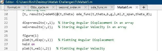
Changing that clears the Error.

Results:

The output obtained is graphical representation velocity curve and displacement curve w.r.t Time.

The animation of the Pendulum motion:

https://youtu.be/4qC9dKP5IMs

Conclusion:

• We have animated the simple pendulum using the ode45 solver where the second order is reduced to a simple differential equation where it is easy to solve the given equation.
• The animation is made using the different points of the bob and the motion of the simple pendulum is created.

References:

https://mathinsight.org/ordinary_differential_equation_introduction#:~:text=An%20ordinary%20differential%20equation%20(ODE,or%20functions%20satisfy%20the%20equation.&text=In%20general%2C%20solving%20an%20ODE%20is%20more%20complicated%20than%20simple%20integration.

https://www.school-for-champions.com/science/pendulum_equations.htm

https://services.math.duke.edu/education/ccp/materials/diffeq/pendulum/pend1.html

https://www.tutorialspoint.com/matlab/matlab_functions.htm

https://skill-lync.freshdesk.com/support/solutions/articles/43000580976-understanding-ode45

https://skill-lync.freshdesk.com/support/solutions/articles/43000580974

https://www.tutorialspoint.com/matlab/matlab_for_loop.htm