Project 1 - Parsing NASA thermodynamic data
AIM: To write a program in matlab to parse the NASA thermodynamic data file and then calculate the thermodynamic properties of various gas species.
OBJECTIVE:
- To write a function that extracts the 14 co-efficients from THERMO.dat file and calculate the enthalpy, entropy and specific heats for all species in the data file.
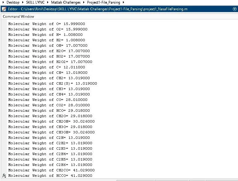
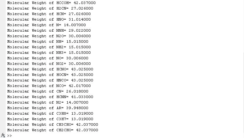
- Calculating the molecular weight of each species and displaying it in command window.
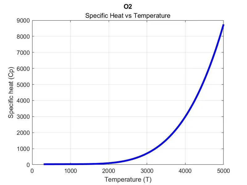
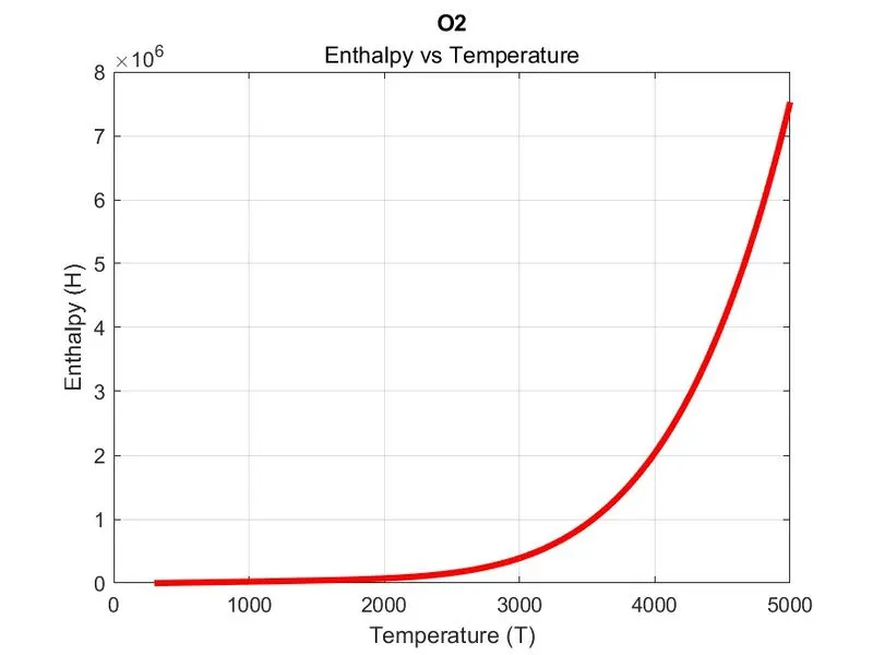
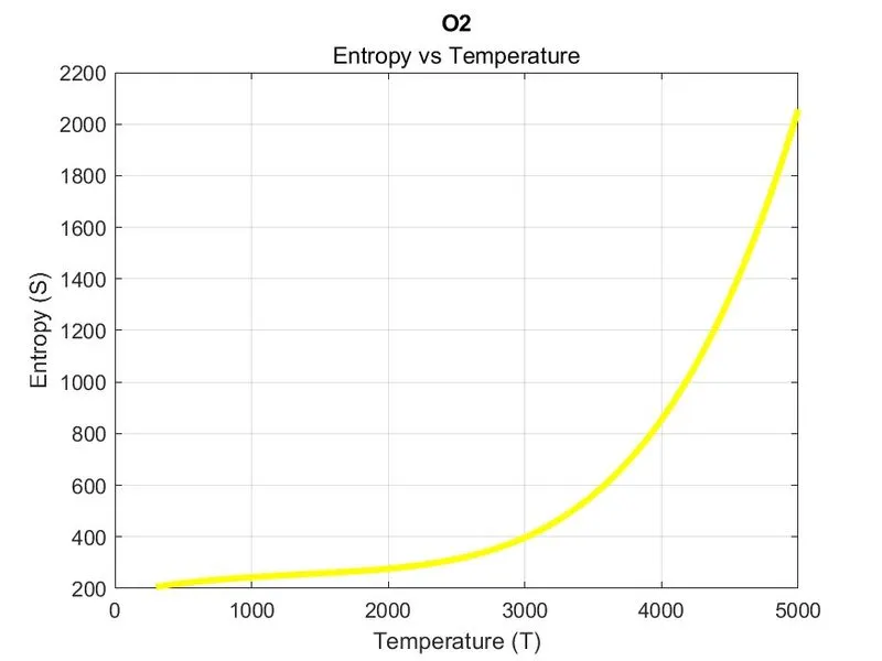
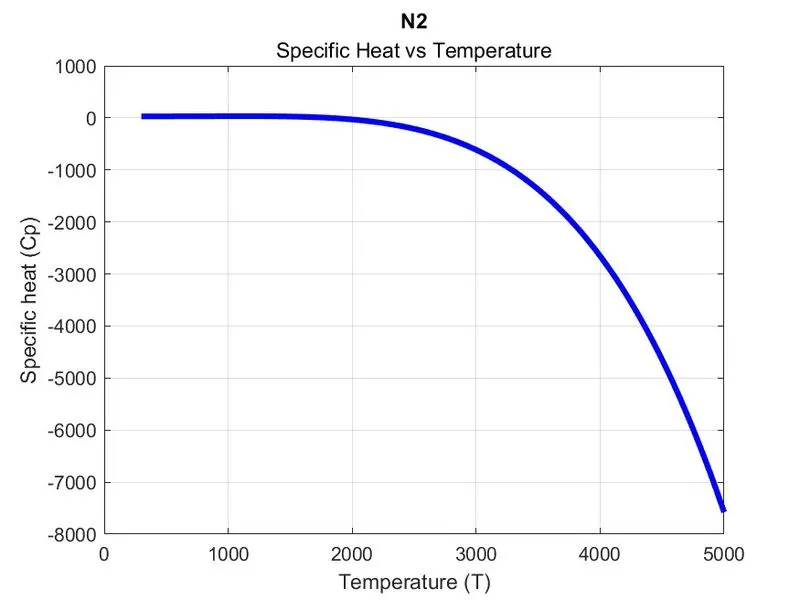
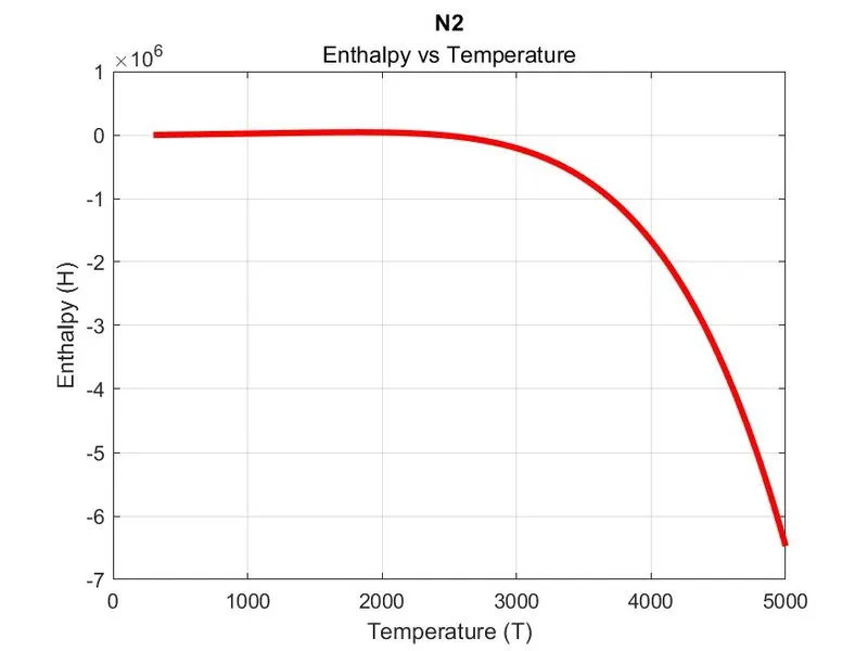
- Plotting Cp, enthalpy and entropy for local temperature range specific for each species.
- Save the plot as images with appropriate names and dump them in separate folders for each species with suitable name.
INTRODUCTION:
PARSING DATA:
Parsing means to make something understandable. For programming this means to convert information represented in one form into another form that's easier to work with. This is done by partially analysing the data, understanding its underlying structure (by making some assumptions based on what you're expecting to see), and then explicitly representing that structure in the code.
Parsing a file means reading in a data stream of some sort and building an in memory model of the semantic content of that data. This aims at facilitating perfoming some kind of transformation on the data.
NASA Thermodynamic File:-
NASA thermodynamics file which is THERMO.dat file in which there are temperature range and 53 species are given in these data and each species contains 14 coefficients and temperature ranges and we have to parse these 14 coefficients to find Specific heat, Entropy and Enthalpy using the following equations:
EQUATIONS:
`(C p)/ R = a _1 + a _2 T + a _3 T^ 2 + a_ 4 T^ 3 + a_ 5 T^ 4`
`(H R)/ T = a _1 + (a_ 2 T)/2 + (a _3 T ^2)/ 3 + (a _4 T^ 3)/ 4 + (a_ 5 T^ 4)/ 5 + a _6 /T`
`S /R/= a _1 ln T + a _2 T + (a _3 T^ 2)/ 2 +( a_ 4 T^ 3)/ 3 + (a _5 T^ 4 )/4 + a 7`
where,
R = Universal Gas constant
T = Temperature
Cp = Specific heat
S = Entropy
H = Enthalpy
Specific Heat:-
The specific heat is the amount of heat per unit mass required to raise the temperature by one degree Celsius.
Entropy:-
- First we write the main code and then we write the calling functions for the properties of individual species from THERMO.dat file such as Specific Heat (Cp), Enthalpy (H), Entropy (S) and Molecular Weight.
- In the main code we extract global temperatures, each species and their polynomial coeffiecients and their local temperatures from the NASA file.
- Then we pass them to calling functions.
- Here we are using two functions one for Cp,H and S collectively and the other for Molecular Weight.
- Cp, H and S are calculated using the given formulae in the function code.
- Molecular Weight function is calculated using for loops and if statements and the atomic weight of the main elements in the species such as Hydrogen (H), Carbon (C), Oxygen (O), Nitrogen (N) and Argon (A).
- We print the Molecular weight in the command window for each species in the main code.
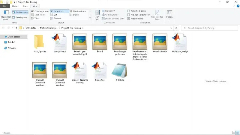
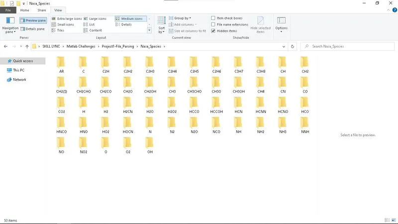
- Then we plot the required figures for each species, save them in individual folders and place them in a parent folder called ' NASA_Species '.
MAIN CODE:
% MATLAB PROJECT 1 - PARSING NASA THERMODYNAMIC DATA

% Main Program

% clearing all previous stored values and clearing command window
clear all
close all
clc

% Creating a new Folder to store the output
mkdir Nasa_Species
R=8.314; % Molar Gas Constant

% Opening and reading THERMO.dat file
f1= fopen('THERMO.dat','r'); % Open and reading THERMO.dat file

% Skipping the first line
fgetl(f1); % Line 1

line2=fgetl(f1); % Line 2 assigned to a variable to extract further data
line2_split=strsplit(line2,' '); % using strsplit to split each value by separating from the spaces
                                 % this variable is now a cell array

% Accessing each value from the cell array and storing into separate variables
% Global Temperatures
global_low_temp=str2num(line2_split{2});
global_mid_temp=str2num(line2_split{3});
global_high_temp=str2num(line2_split{4});

% Temperature range
T=linspace(global_low_temp,global_high_temp,1000);

% Skipping the next 3 lines
fgetl(f1); % Line 3
fgetl(f1); % Line 4
fgetl(f1); % Line 5

%% Reading Species, Calcuating Cp,H,S,MW and Plotting

for i=1:53 % for 53 species

    tline=fgetl(f1);

    A=strsplit(tline,' ');  % Splitting the line to cell array
    name_of_species=(A{1}); % Getting the name of the species

    lowtemp=str2num(A{end-3}); % Getting the low tempeature
    midtemp=str2num(A{end-2}); % Getting the low tempeature
    hightemp=str2num(A{end-1}); %Getting the low tempeature

    % Finding 7 higher and 7 lower coefficients

    tline1=fgetl(f1);
    a=findstr(tline1,'E'); % Finding the indices/indexes of character E

    a1=tline1(1:a(1)+3); % First value
    a1=str2num(a1); % Changing the string value to numerical value
    a2=tline1(a(1)+4:a(2)+3);
    a2=str2num(a2);
    a3=tline1(a(2)+4:a(3)+3);
    a3=str2num(a3);
    a4=tline1(a(3)+4:a(4)+3);
    a4=str2num(a4);
    a5=tline1(a(4)+4:a(5)+3);
    a5=str2num(a5);

    tline2=fgetl(f1);
    a=findstr(tline2,'E');

    a6=tline2(1:a(1)+3);
    a6=str2num(a6);
    a7=tline2(a(1)+4:a(2)+3);
    a7=str2num(a7);
    a8=tline2(a(2)+4:a(3)+3);
    a8=str2num(a8);
    a9=tline2(a(3)+4:a(4)+3);
    a9=str2num(a9);
    a10=tline2(a(4)+4:a(5)+3);
    a10=str2num(a10);

    tline3=fgetl(f1);
    a=findstr(tline3,'E');

    a11=tline3(1:a(1)+3);
    a11=str2num(a11);
    a12=tline3(a(1)+4:a(2)+3);
    a12=str2num(a12);
    a13=tline3(a(2)+4:a(3)+3);
    a13=str2num(a13);
    a14=tline3(a(3)+4:a(4)+3);
    a14=str2num(a14);

    % Function Calling
    % Calculating Specific Heat(Cp), Enthalpy(H), Entropy(S)
    [Cp,H,S] = Properties(a1,a2,a3,a4,a5,a6,a7,a8,a9,a10,a11,a12,a13,a14,R,T,global_mid_temp);

    % Calculating Molecular Weight and printing
    MW = Molecular_Weight(name_of_species);
    fprintf('Molecular Weight of %s= %f\n',name_of_species,MW);

    % Changing the directory to Sub Folder Nasa_Species
    cd Nasa_Species
    mkdir(name_of_species); % Creating subfolder for each species with names
    cd(name_of_species); % Changing current folder to species folder


    % Plotting CP,H,T

    % Plotting Cp vs T
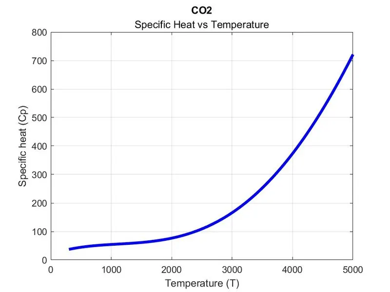
    figure(1)
    plot(T,Cp,'linewidth',3,'Color','b');
    xlabel('Temperature (T)');
    ylabel('Specific heat (Cp)');
    title(name_of_species, 'Specific Heat vs Temperature')
    grid on
    saveas(figure(1),'Specific Heat.jpg') % Saving the plot as JPG file

    % Plotting H vs T
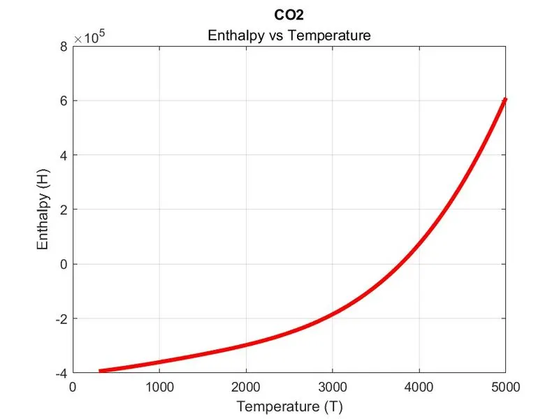
    figure(2)
    plot(T,H,'linewidth',3,'Color','r');
    xlabel('Temperature (T)');
    ylabel('Enthalpy (H)');
    title(name_of_species, 'Enthalpy vs Temperature')
    grid on
    saveas(figure(2),'Enthalpy.jpg')

    % Plotting S vs T
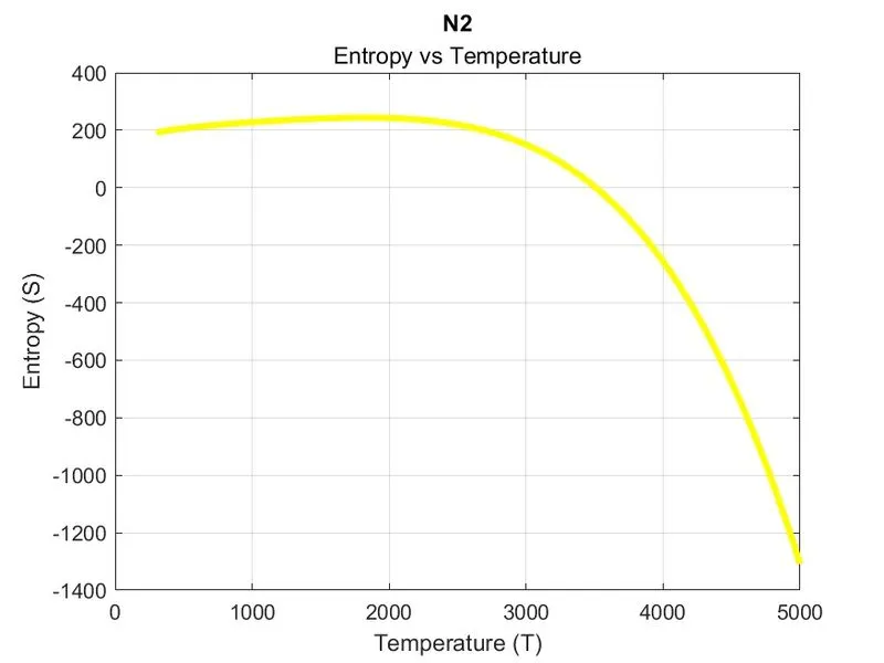
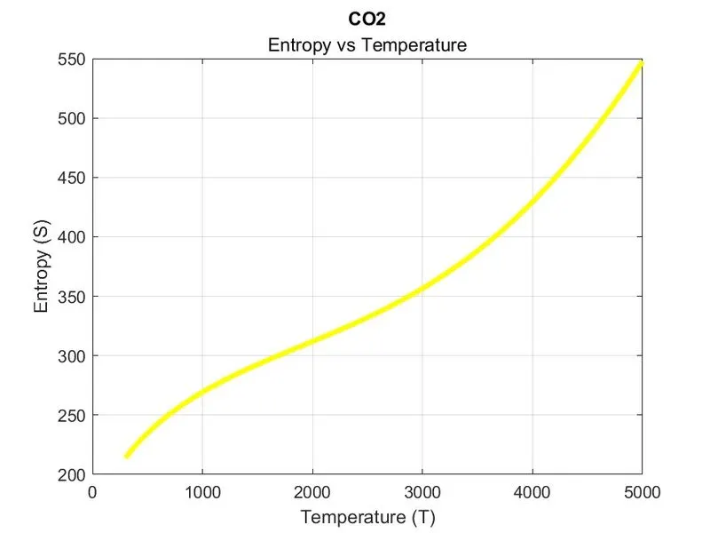
    figure(3)
    plot(T,S,'linewidth',3,'Color','y');
    xlabel('Temperature (T)');
    ylabel('Entropy (S)');
    title(name_of_species, 'Entropy vs Temperature')
    grid on
    saveas(figure(3),'Entropy.jpg')

    % Changing back to Parent Folder
    cd('C:\Users\Rinil\Desktop\SKILL LYNC\Matlab Challenges\Project1-File_Parsing')

end
Function for Specific Heat, Enthalpy and Entropy:
% Specific Heat, Enthalpy and Entropy function
% for lower or higher temperarures

function [Cp,H,S] = Properties(a1,a2,a3,a4,a5,a6,a7,a8,a9,a10,a11,a12,a13,a14,R,T,global_mid_temp)

if(T>=global_mid_temp)
    Cp=R*(a1+(a2*T)+(a3*(T).^2)+(a4*(T).^3)+(a5*(T).^4));
    H=R*((a1*T)+((a2*(T).^2)/2)+((a3*(T).^3)/3)+((a4*(T).^4)/4)+((a5*(T).^5)/5)+a6);
    S=R*(a1.*log(T)+(a2*T)+((a3*(T).^2)/2)+((a4*(T).^3)/3)+((a5*(T).^4)/5)+a7);
else
    Cp=R*(a8+(a9*T)+(a10*(T).^2)+(a11*(T).^3)+(a12*(T).^4));
    H=R*((a8*T)+((a9*(T).^2)/2)+((a10*(T).^3)/3)+((a11*(T).^4)/4)+((a12*(T).^5)/5)+a13);
    S=R*(a8.*log(T)+(a9*T)+((a10*(T).^2)/2)+((a11*(T).^3)/3)+((a12*(T).^4)/4)+a14);
end
end
% Molecular Weight Function

function W = Molecular_Weight(name_of_species)

    % Defining Atomic name of the main elements in the species list
    atomic_name = ['H','C','O','N','Ar'];

    % Defining Atomic masses of the main elements
    atomic_weight = [1.008 12.011 15.999 14.007 39.948];

    % Molecular weight starting range
    W = 0;
    species = name_of_species;

    for i=1:length(species)   % Loop runs to the length of the species
        for j=1:length(atomic_name)  % Loop runs to the length of the atomic names
            if strcmp(species(i), atomic_name(j))  % Function to compare 2 strings
                W = W + atomic_weight(j);
                position = j;
            end
        end

        % Finding if there is more elements in the species
        n = str2num(species);

        if n>1
            W = W + atomic_weight(position)*(n-1);  % Incrementing the atomic weight of the extra element
        end
    end

end
CODE EXPLANATION:
- First we create a new folder ' NASA_Species ' in the current folder using mkdir function.
- The value of Gas Constant ‘R’ is defined as R=8.314 .
- Then we use fopen command to open the file ‘ THERMO.dat ’ .
- Next we use the fgetl to read the first line. Using the same command gives you the second line. without assigning to a variable the command is used to skip a line. Now we are in the second line which has the global temperatures.
- We use the strsplit command to split each value( with space in between ) in that line to a cell array. Infact using strsplit returns a cell array.
- Now we convert the strings to numbers using the str2num command and assigning global (low,mid and high) temperatures to each individual variables.
- Then we have written a command to get the temperature range for calculation and plotting purpose.
- Then again using the fgetl command to go to skip the next 3 lines.
- Then we use a for loop to get 53 species and their local temperatures (low, mid, high) and the 14 coefficients.
- In the for loop we again use the fgetl command and then the next line is read and from that line the species name, the three local temperatures are read and stored.
- Then we use fgetl command to go to further line and get the first 7 coefficients and store them. Similarly using the fgetl command we move to the next two lines and get the remaining coefficients.
- Then after getting the 14 coefficients, we use these coefficients and by calling the functions we calculate Cp,H,S.
- Further we use the Molecular weight function and calculate molecular weight for that species andd print it in the main code.
- Next we change the directory so that we can save the files at that particular location. We use the cd command to go into the sub folder NASA_Species from the current folder.
- After changing the directory we use mkdir command again to create a new folder with the name of the current species and then a cd command again to make the newly created folder as the current directory.
- Now we use plot command to plot Temperature vs (Specific Heat, Enthalpy, Entropy) .
- In this plotting we use the figure command to get the three different plots and saveas command to save the figures in the folder.
- Then we change our directory again to the very first parent folder to start the loop. So the loop continues to function till we get all the 53 species and then it gets terminated.
ERRORS:
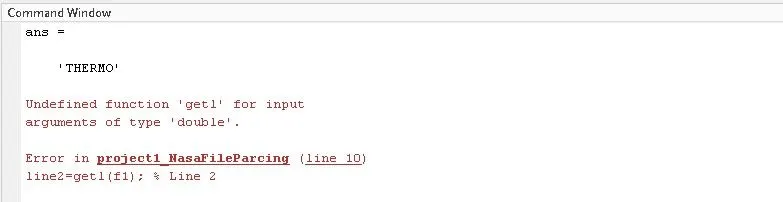
1. Used getl instead of fgetl command to get the line from the file.
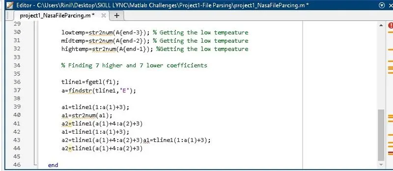
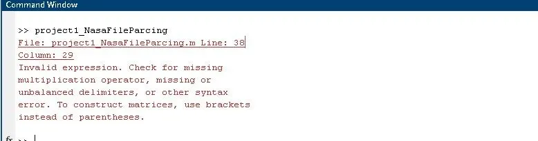
2. Copy paste error. The code was not complete. Hence i had to complete the code and execute.
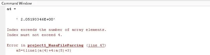
3. Because I didnt complete coding for 6-14 coefficents in the for loop. Hence executing the code with incomplete code gave error. Had to complete and execute.
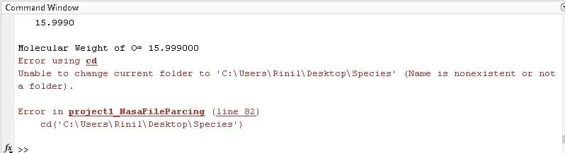
4. cd error. Changing directory syntax was wrong completely. Used a completely different way for the folder part of this project.
FINAL RESULTS:
Output for Molecular Weight:-
SCREENSHOTS:
PLOTS:
Plots for `O_2`
Plots for `N_2`
Plots for `CO_2`
Parent Folder:
Species Folder:
CONCLUSION:
Using MATLAB, the necessary coefficients required to evalute various thermodynamic parameters for different species are extracted from the THERMO.dat file. The specific heat, entropy and enthalpy for all the species are calculated and plotted against the temperature range. They are saved to each individual species folder inside parent folder called NASA_Species. The molecular weight is calculated for all the species and displayed.
Therefore, we have successfully parsed the given NASA thermodynamic data file.
REFERENCES:
https://en.wikipedia.org/wiki/Parsing
https://www.wikihow.com/Calculate-Molecular-Weight
https://www.me.psu.edu/cimbala/learning/general/gas_constant.pdf
https://ntrs.nasa.gov/api/citations/19720021272/downloads/19720021272.pdf
https://www.mathworks.com/matlabcentral/answers/317006-create-new-folders-by-mkdir
https://www.mathworks.com/matlabcentral/answers/17580-how-to-define-a-path-in-saveas-command
https://www.mathworks.com/matlabcentral/answers/106320-make-a-loop-to-calculate-molecular-weight