Week 5 - Genetic Algorithm

Genetic Algorithm:

Theory:

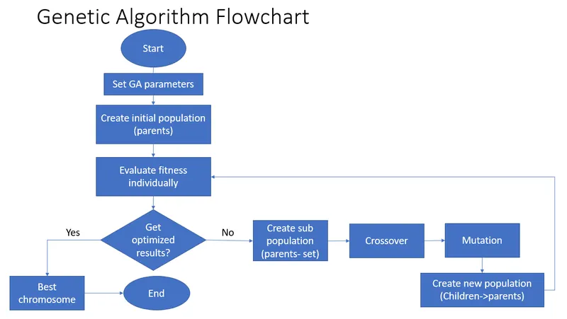
Genetic Algorithm is a method which is used in order to search a solution space for an optimal solution for a problem inspired by Charles Darwin theory of evolution. Darwinian Theory of Evolution explains that evolution is the result of natural selection, and natural selection is biased by the inherited characteristics of organisms. The adaptive ability of organisms is the one which helps organisms in evolution through natural selection. The genetic algorithm reflects the process of natural selection where the fittest individuals(as parents) are selected for reproduction in order to produce offspring of the next generation.In operations research , this algorithm is commonly used to generate high-quality solutions to optimation and search problems by relying on biologically inspired operators such as mutations, crossover and selection

Steps:

Five set are consider in a Genetic Algorithm.

1. Initial population
2. Fitness function
3. Selection
4. Crossover
5. Mutation
6. Termination

Flowchart:

Matlab Code:

Defining inputs:

Input:

clear all
close all
clc

% defining search space
x = linspace(0,0.6,150);
y = linspace(0,0.6,150);
num = 40;   % number of times ga runs

% creating a 2D mesh
[xx, yy] = meshgrid(x,y);

Explanation:

Here, we used the linspace() function to define the input variables. The syntax for linspace is:

linspace(start_variable:end_variable:number_of_variables)

If number of variables is not defined then we get 100 evenly spaced elements.

(x_2d,y_2d) = meshgrid(x_var,y_var) returns 2-D grid coordinates based on the coordinates contained in vectors x and y. x_2d is a matrix where each row is a copy of x, and y_2d is a matrix where each column is a copy of y.

Stalgmite function:

Theory:

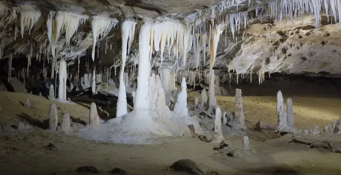
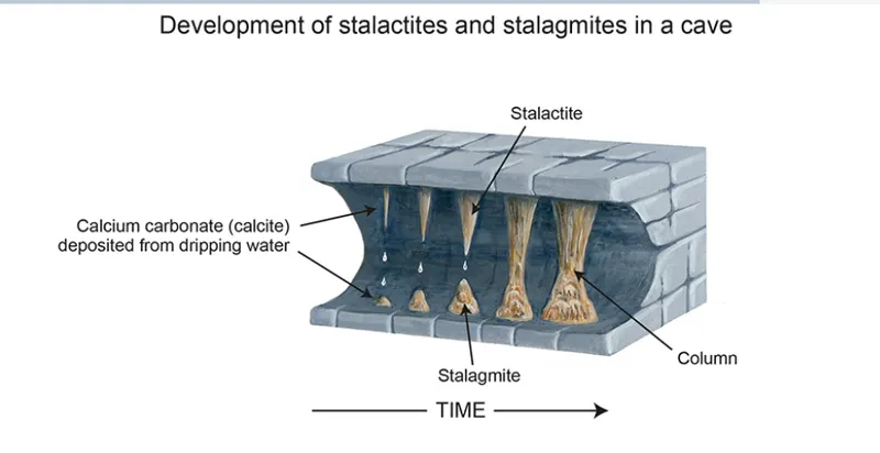
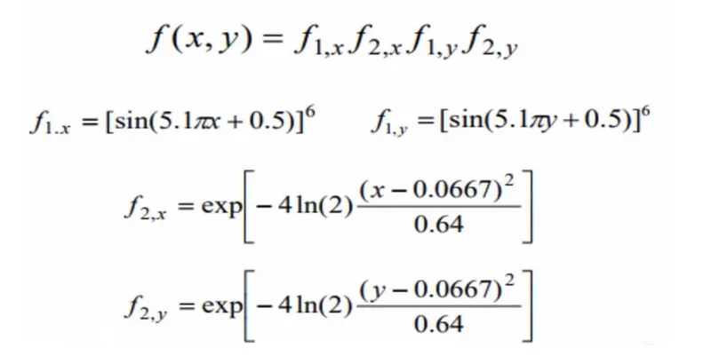
A stalagmite is an upward-growing mound of mineral deposits that have preciptated from water dripping onto the floor of a cave. The stalagmite function uses the data to create stalagmites.

Mathematical Formula:

The mathematical formula to create stagmite plot is given below:

Function definition:

Input:

% stalagmite function

function [output] = stalagmite(input_vector)
  a = input_vector(1);
  b = input_vector(2);
  
  f1x = (sin(5.1*pi*a+0.5))^6;
  f1y = (sin(5.1*pi*b+0.5))^6;
  f2x = exp(-4*log(2)*(a-0.0667)^2/0.64);
  f2y = exp(-4*log(2)*(b-0.0667)^2/0.64);
  
  [output] = -(f1x*f2x*f1y*f2y);
end

Explanation:

The stalagmite function is used to create a stalagmite using the values of mesh values.

The syntax to define function is:

function function_name(input_variable)

statement-1;

statement-1;

return_variable=value;

return;

endfunction

Care should be taken that the 'file name ' should be same as the 'function name'.

Function calling:

Input:

% evaluating the stalagmite function

for j = 1:length(xx)
  for k = 1:length(yy)
    input_vector(1) = xx(j,k);
    input_vector(2) = yy(j,k);
    f(j,k) = stalagmite(input_vector);
  end
end

Explanation:

The syntax of 'for' loop

for(start_value:end value)

statement;

end

length(input_array)= number of elements in the array.

The syntax to call a function is:

output_variable=function_name(input_variable)

Case-1:Genetic Algorithm(Unbounded_Inputs)

Input Code:

% study 1 : statistical behaviour

tic
for l = 1:num
[input_1, fopt_1(l)] = ga(@stalagmite,2);
xopt_1(l) = input_1(1);
yopt_1(l) = input_1(2);
end
study_time_1 = toc;

Explanation:

The syntax of 'for' loop

for(start_value:end value)

statement;

end

We have defined ‘x’ & ‘y’ values and then we have decide the number of times the ‘ga ()’ has to be performed as a variable “num_case” and we have given it a value. Now using the For Loop value of “f_opt” are determined, it is same as the above code used in this “FOR LOOP”.Now since the value of ‘f’ is negative and we get the downward graph ,so in order to get upward graph ,we have multiplied ‘f’ with “-“(minus) symbol and assigned it to variable “F”.Now here another FOR LOOP is used to evaluate “ga ()” for 40 iterations we have defined “l” as the number of iteration and then we have entered the “ga ()" function with the normal syntax that we have mention in previous code. Only the fitting function and number of variable are entered as inputs for the “ga ()” function.

Graph-1:

Input:

figure(1)
subplot(2,1,1)
hold on
surfc(xx, yy, -f)
shading interp
plot3(xopt_1,yopt_1,-fopt_1,'marker','o','markersize',5,'markerfacecolor','r')
title('Unbounded inputs')
xlabel('X values')
ylabel('Y values')
subplot(2,1,2)
plot(-fopt_1)
xlabel('Iterations')
ylabel('Function Maximum')

Explanation:

We use surfc() to show the stalgamite in 3d and plot3() to show the values in 3d format.

subplot is used to show multiple plots. The syntax of subplot is

subplot(row_num,column_num_graph_num).

Output:

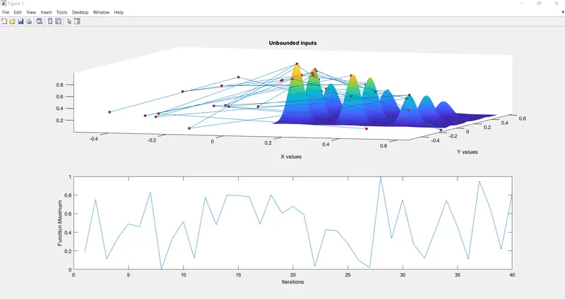
Observations:

We can observe that we have got different optimized values of function “f” each the “ga ()” was run.

We have got 40 different value of “f” when 40 times “ga ()” was run. The values of “f” are changing for each iteration. GA always take random population sample and then perform the mutation and crossover process to get a new generation. Due to this random inputs taken by genetic algorithm we get the different value when we run the “ga ()” each time .Here genetic algorithm does not know what is our search space i.e. limits of ”x” and “y”

Case-2:Genetic Algorithm(Bounded_Inputs)

Input Code:

% study 2 : statistical behaviour with upper and lower bounds

tic
for l = 1:num
[input_2, fopt_2(l)] = ga(@stalagmite,2,[],[],[],[],[0;0],[1;1]);
xopt_2(l) = input_2(1);
yopt_2(l) = input_2(2);
end
study_time_2 = toc;

Explanation:

The syntax of 'for' loop

for(start_value:end value)

statement;

end

Now in this code the syntax used for “ga ()” command is

X = ga(fun,nvars,A,b,Aeq,beq,lb,ub)

define a set of lower and upper bounds on the design variable,x,so solution is found between the range (Set A = [] and b = [] if no linear inequalities exist.) (Set Aeq = [] and beq = [] if no linear equalities exist). The above syntax help us to enter upper and lower bound value as input to get the better solution than previous code. This means that when “ga()” calculates the value of ”f” ,it will display on the value of “f” that lies between the bounded values of “x” and “y”. Now it is not compulsory to take the values of “x” and ”y” values only as your bounded values , these values are taken according to the problem we are working on , sometimes for the bounded values to be specified need some practical experience for some situations .So bounded values are taken according to our problem.

Graph-2:

Input:

figure(2)
subplot(2,1,1)
hold on
surfc(xx, yy, -f)
shading interp
plot3(xopt_2,yopt_2,-fopt_2,'marker','o','markersize',5,'markerfacecolor','r')
title('Bounded inputs')
xlabel('X values')
ylabel('Y values')
subplot(2,1,2)
plot(-fopt_2)
xlabel('Iterations')
ylabel('Function Maximum')

Explanation:

We use surfc() to show the stalgamite in 3d and plot3() to show the values in 3d format.

subplot is used to show multiple plots. The syntax of subplot is

subplot(row_num,column_num_graph_num).

Output:

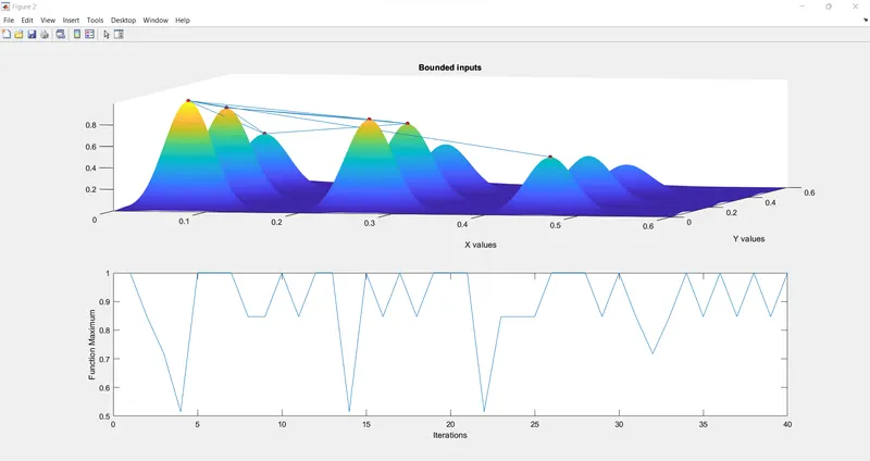
Observations:

We can observe that now the graph is much better clear then previous one and now –ga() predict that the global maxima is somewhere between three points that are in first plot. Second value is between 0.6 to 1. But here we still didn’t get the optimized value ,i.e results are yet not clear. To overcome this problem , further we are using modified “ga ()” command.

Case-3:Genetic Algorithm(Bounded_Inputs_different poupation)

Input Code:

% study 3 : increasing GA population size

options = optimoptions('ga');
options = optimoptions(options,'PopulationSize',450);

tic
for l = 1:num
[input_3, fopt_3(l)] = ga(@stalagmite,2,[],[],[],[],[0;0],[1;1],[],[],options);
xopt_3(l) = input_3(1);
yopt_3(l) = input_3(2);
end
study_time_3 = toc;

Explanation:

The syntax of 'for' loop

for(start_value:end value)

statement;

end

In this code after the fitting function is calculated , we have a command called “optimoptions()”, the syntax for this command is

Options = optimoptions(SolverName)returns a set of default options for the SolverName solver.

Options = optimoptions(SolverName,Name,Value) return options with name parameters altered with the specified values.

If we increase the value of “PopulationSize” then “ga” will have more samples tp choose and perform mutation and cross-over then it can give us more accurate optimized value.

Graph-3:

Input:

figure(3)
subplot(2,1,1)
hold on
surfc(xx, yy, -f)
shading interp
plot3(xopt_3,yopt_3,-fopt_3,'marker','o','markersize',5,'markerfacecolor','r')
title('Bounded inputs with different population size')
xlabel('X values')
ylabel('Y values')
subplot(2,1,2)
plot(-fopt_3)
xlabel('Iterations')
ylabel('Function Maximum')

Explanation:

We use surfc() to show the stalgamite in 3d and plot3() to show the values in 3d format.

subplot is used to show multiple plots. The syntax of subplot is

subplot(row_num,column_num_graph_num).

Output:

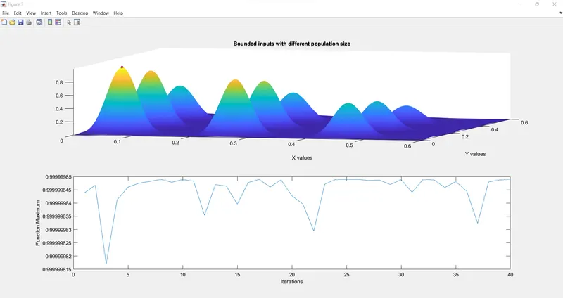
Observations:

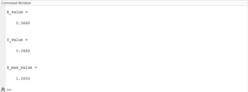
We can observe that by increasing the population size we have got a single optimized value in the 1^st graph . If we increase the population size more further, the value will be more accurate .The maximum value of for many iteration is near to 0.9999985, So the maximum value is somewhere near to this value.

Finding the max value:

Code:

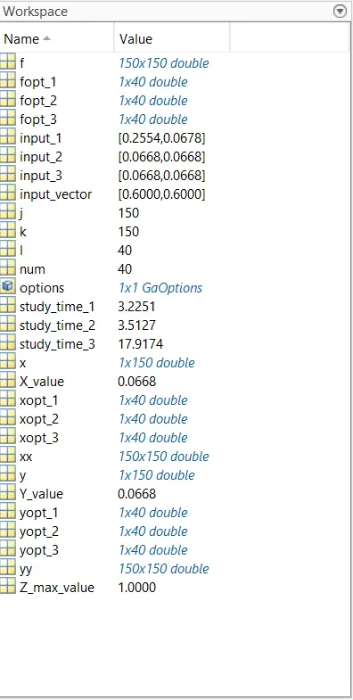
X_value = input_3(1)
Y_value = input_3(2)
Z_max_value = max(-fopt_3)

Output:

Workspace: