Week 4.1 - Solving second order ODEs

Objective:

Write a program that solves the following ODE. This ODE represents the equation of motion of a simple pendulum with damping.

In the above equation,

g = gravity in m/s2,

L = length of the pendulum in m,

m = mass of the ball in kg,

b=damping coefficient.

Write a program in Matlab\Octave that will simulate the pendulum motion, just like the one shown in the start of this challenge.

use,

L=1 metre,

m=1 kg,

b=0.05.

g=9.81 m/s2.

Simulate the motion between 0-20 sec, for angular displacement=0,angular velocity=3 rad/sec at time t=0

Input:

%progranm to find the second order derivations
close all
clear all
clc

% define constants

b = 0.05;
g = 9.81;
l = 1;
m = 1;

%intial condition

theta_0 = [0;3];

%time points

t_span = linspace(0,20,500);

Explanation:

The inputs are given in the question . For the time span, we use the linspace() function. the linspace() function returns evenly spaced variables.

The syntax is:

linspace(start_val,end_val,number of variables)

if the number of variables is not given then the function returns 100 evenly spaced variables.

The matrix theta gives Angular displacement and angular velocity.

`theta = theta_1` angular displacement.

`d(theta)/dt = theta_2` angular velocity.

ODE45:

Explanation:

The ode45 differential equaltion solver. ode full form is ordinary differential equation. ode 45 takes the input variables and calls a function to solve differential equation using a Runge-Kutta method. Runge–Kutta method used for solving the initial-value problems of differential equations. The syntax for ode45 is

[time_output, output_var_1_array] = ode45(@diff_func_name(fun_time_input,input_1,...input_n), time_span_array_input, input_var_1_array)

Function defination:

Input:

function [dtheta_dt] = ode_func(t,theta,b,g,l,m)

  theta1 = theta(1);
  theta2 = theta(2);
  dtheta1_dt = theta2;
  dtheta2_dt = -(b/m)*theta2 - (g/l)*sin(theta1);
  dtheta_dt = [dtheta1_dt; dtheta2_dt];
  end

Explanation:

The ode45 deals with first order differential eqautions, so we need to convert the second order differential equations to series of first order differential eqautiond. To convert the differential eqautions, we need to create a function.

The syntax for a function is:

function [return_var] = function_name(input_var_1,input_var_2...input_var_n)

statement_1;

statement_2;

end

The way to convert the differential equations is:

`theta = theta_1` is angular displacement.

`d(theta)/dt = theta_2` is angular velocity.

`d^2(theta)/dt^2 = -(b/m)*theta_2 -(g/L)*sin(theta_1)`

through these steps, the second order equation is converted into a series of first order equations.

Function calling:

Input:

% call the second order function

[t,results] = ode45(@(t,theta)ode_func(t,theta,b,g,l,m),t_span, theta_0);

Explanation:

Through ode45 we call the function.

The syntax for ode45 is

[time_output, results_array] = ode45(@diff_func_name(time_input,input_1,...input_n), time_span_array, input_1_array)

here we are specifying that the time_span and input array are the variables that the differential equations are based on.

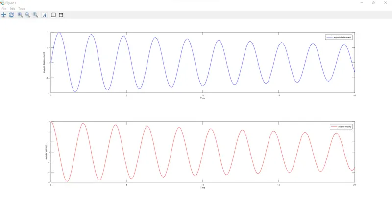
Plot the Graphs

Input:

%plot the graphs
figure(1)

subplot(2,1,1)
plot(t,results(:,1),'color','b');
legend('angular displacement');
ylabel('angular displacement');
xlabel('Time');
hold on
subplot(2,1,2)
plot(t,results(:,2),'color','r');
legend('angular velocity');
ylabel('angular velocity');
xlabel('Time');

Explanation:

We can use the plot() function to plot the graphs. the syntax for plot() function is:

plot(x_val, y_val)

color: b = blue, r = red

legend('legend-string')

xlabel('x-axis-string')

ylabel('y-axis-string')

Using subplot() function, we can have more than one graph in the figure. the syntax for the subplot() is:

subplot(number of rows, number of coloumns, number of graph)

Graphs:

Creating the Animation:

Input:

figure(2)

%animation
THETA = results(:,1);
ct = 1;

for j = 1:length(THETA)
  THETA_1 = THETA(j);
  x0 = 0;
  y0 = 0;

  x1 = l*sin(THETA_1);
  y1 = -l*cos(THETA_1);
  plot([-0.5,0.5],[0,0],'linewidth',4,'color','b');
  hold on
  line([x0 x1],[y0 y1],'linewidth',2,'color','k');
  hold on
  plot(x1,y1,'marker','o','markersize',12,'markerfacecolor','r');
  hold off
  grid on
  axis([-2 2 -2 1.5]);
  title("Pendulam");
  pause(0.04);
  frame = getframe(gcf);
  im = frame2im(frame);


    if ct == 1;
          % Create GIF file
          imwrite(im,'animation_6.gif','gif','DelayTime', 0.04, 'Compression' , 'lzw');
      else
          % Add each new plot to GIF
          imwrite(im,'animation_6.gif','gif','WriteMode','append','DelayTime', 0.04 , 'Compression' , 'lzw');
      end

    ct=ct+1;
endfor

Explanation:

Animation is collection of images stitched together. So we have to save every plot. And then save all the plot to create a gif.

To create the gif file we use for() loop. the syntax is

for condtion

statement

end

here the condition is j = 1 to length of array

the length() function is used find the length of the array.

The array is results 1 coloumn. angular displacement.

To create the plot we use the plot() function.

Plot each point with respect to theta, 'angular diplacement'.

Using hold on function we keep the plots of the ceiling,the string and pendulum. Then we use hold off to the new plot.

Each plot is captured into frame by getframe() function. gcf captures the current frame.

The frame is converted into image using the frame2im() function.

the using the if loop we create and modify the gif. the syntax is:

if condition

statement_1-------------------> condition is true

esle

statement_2-------------------> condition is false

To create the gif we use imwrite() function. the syntax used is

imwrite(image_input,'filename','file_type','delay time','delay time value','compression','compression type')

And then we have to add new images to the file. we use imwrite() function again, but in write mode. the syntax is:

imwrite(image_input,'filename','file_type','write mode', 'append','delay time','delay time value','compression','compression type')

here the image input is the image of the current frame

file name is 'animation-6.gif'

file type is 'gif'

delay time is 20/500 = 0.04 sec

compression type is = lzw

Output:

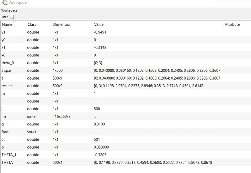
Workspace:

Errors:

1. String and ceiling is not plotted

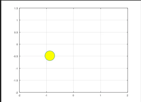
2. The plots overlapped.

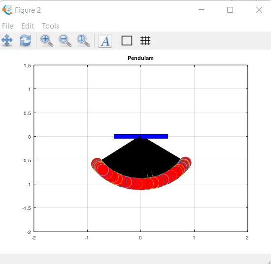
Solution:

1.To show the ceiling and the string along with the pendulum, we have to use 'hold on' command

2. To avoid overlapping, we need to use 'hold off' function.