Project 1 - Parsing NASA thermodynamic data
Objective:
1. Write a function that extracts the 14 co-efficients and calculates the enthalpy, entropy and specific heats for all the species in the data file. The formulae are shown below.
Here R is the universal gas constant, T is the temeprature
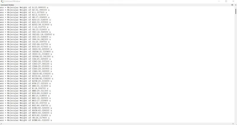
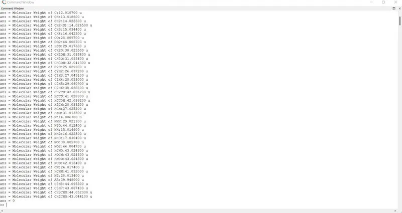
2. Calculate the molecular weight of each species and display it in the command window.
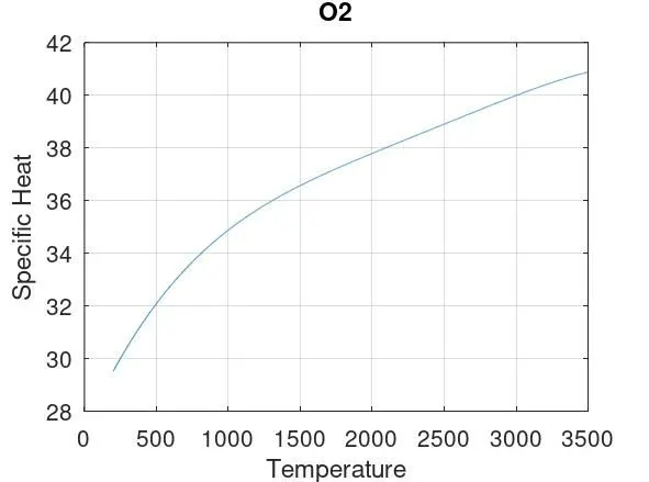
3. Plot the Cp, Enthalpy and Entropy for the local temperature range (low temperature : high temperature) specific for each species.
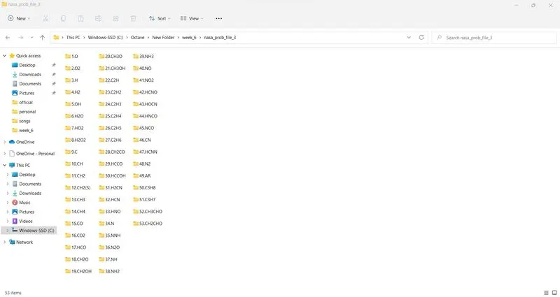
4. Save the plots as images with appropriate names and dump them in separate folders for each species with suitable name. All these should be generated automatically.
Program:
Read the file 'NASA thermodynamic data'. Extract the data from the file and exetute the he values in the formulea to find the results.
Opening the data file:
Code:
clear all
close all
clc

f3 = fopen('THERMO.dat','r');
Explanation:
The File must be opened. We use the fopen funtion. the syntax for fopen function is:
file_id = fopen('filename','permission')
here permission can be to write a file(w) or to read a file(r) or to append a file(a).
Extracting the data:
Code:
heading_tline = fgetl(f3);

tline_2 = fgetl(f3);

A = strsplit(tline_2,' ');

global_low_temp = str2num(A{2});
global_mid_temp = str2num(A{3});
global_high_temp = str2num(A{4});

comment_tline_3 = fgetl(f3);
comment_tline_4 = fgetl(f3);
comment_tline_5 = fgetl(f3);
Explanation:
Now, that we have opend the file we have to read the data from the file. To do that we use fgetl() function. The fgetl() function reads a line from the data file, removing any newline characters. The syntax for fgetl() is
line_string = fgetl(file_id).
Each time we type fgetl() the function reads the next line in the data file.
The second line consists of information regarding the global tempetature. We use the strsplit() function to split the string.The syntax for strsplit() function is
variable = strsplit(string, delimiter)
The split string also gives strings. The string has to be converted into a numerical value. To do that we can use the str2num() function
the syntax for str2num() function is:
var_num = str2num(var_str)
Species Data:
The data file has data of 53 species. We have to extract the data like temperatures and co-efficients of each different species.
Extracting Co-efficients:
Input:
We use 'for' loop to extract data of each species.
The syntax to create 'for' loop is:
for condition
statement-1
statement-2
endfor
For each species, we can use getl() function and strsplit() function to get the species name and local temperatures.
To give the file serial number, we use num2str() to convert the serial number to a string. Then the the 'serial number' string and the 'species name' string is concatenated using the strcat() function.
the syntax for the num2str() function is:
var = num2str(str_var)
the syntax for the strcat() function is:
new_string = strcat('string1','string2')
We use the str2double() function to get the local temperatures from the string. str2double() function works in a simillar manner as str2num() function. The str2double uses SCANF while Str2Num uses eval() function. The syntax for str2double() is also simillar to str2num() function:
num_var = str2double(str_var)
We use the getl() functionto get the co-efficients. The 14 coefficients are in 3 lines . The co-efficients have 'E' in the co-efficient string to represent the co-efficient in float data type.
We use strfind() function to find the index of the 'E'. The strfind() function returns an array of indexes. The syntax of strfind() function is:
array = strfind("string","find_var"). The decimal points are 3 digits, so, using that knowledge we find the 14 co-efficients.
Code:
%reading the species
for j=1:53

    s_heading=fgetl(f3);
    x=strsplit(s_heading,' ');

    species_name=(x{1});
    z=length(x);
    sr_no = num2str(j);
    f_species_name = strcat(sr_no,'.',species_name);

    local_low_temp=str2double(x{z-3});
        local_high_temp=str2double(x{z-2});
            local_mid_temp=str2double(x{z-1});

            t1=local_low_temp;
            t2=local_mid_temp;
            t3=local_high_temp;

            %(a1-a5)
            s_tline_1=fgetl(f3);

            a_1=strfind(s_tline_1,'E');
            a1=str2double(s_tline_1(1:a_1(1)+3));
            a2=str2double(s_tline_1(a_1(1)+4:a_1(2)+3));
            a3=str2double(s_tline_1(a_1(2)+4:a_1(3)+3));
            a4=str2double(s_tline_1(a_1(3)+4:a_1(4)+3));
            a5=str2double(s_tline_1(a_1(4)+4:a_1(5)+3));

            %(a6-a10)
             s_tline_2=fgetl(f3);

            a_2=strfind(s_tline_2,'E');
            a6=str2double(s_tline_2(1:a_2(1)+3));
            a7=str2double(s_tline_2(a_2(1)+4:a_2(2)+3));
            a8=str2double(s_tline_2(a_2(2)+4:a_2(3)+3));
            a9=str2double(s_tline_2(a_2(3)+4:a_2(4)+3));
            a10=str2double(s_tline_2(a_2(4)+4:a_2(5)+3));

            %(a10-a14)
             s_tline_3=fgetl(f3);

            a_3=strfind(s_tline_1,'E');
            a11=str2double(s_tline_3(1:a_3(1)+3));
            a12=str2double(s_tline_3(a_3(1)+4:a_3(2)+3));
            a13=str2double(s_tline_3(a_3(2)+4:a_3(3)+3));
            a14=str2double(s_tline_3(a_3(3)+4:a_3(4)+3));


            %creating folder


    %calculate cp, H, S using coeffecients
    %a1-a7 (high temperature coeffeceints)
    %a8-a14(low temperature coeffecients)


            %plotting the graphs

            %changing the directory and saving the file

             %molecular_mass_calculation


end
Explanation:
Creating new folder for species:
Input:
The plots have to be saved in the a separete folder for each species.
Code:
            %creating folder
            mkdir(['C:\Octave\New Folder\week_6\nasa_prob_file_3\',f_species_name]);
Explanation:
We make the directory if it was not created before. To create the directory we use mkdir() function. The syntax for the mkdir() function is:
mkdir([file_path,fine_name])
Finding The Specific Heat, Enthalpy, Entropy:
Input:
Using the co-efficients we found we need to find the values of Specific heat, Enthalpy and entropy with given formula. The range of temperatures can range from the local low temperature to local high temperature. The temperatures whose value is higher than the local mean temperature will use the co-efficients a1 to a7 while the temperatures whose value is lower than the local mean temperature will use the co-efficients a7 to a14. We also assign the value of R as 8.314.
Code:
            T=linspace(t1,t3,1000);
            R=8.314;
            % to get array of specific heat, enthalpy and entropy
            for k=1:length(T)

    %a1-a7 (high temperature coeffeceints)
    %a8-a14(low temperature coeffecients)
    if T(k)>t2

        %high temperature coeffeceints.

        cp=(a1+a2.*T+a3.*T.^2+a4.*T.^3+a5.*T.^4)*R;

        H=(a1+(a2.*T)/2+(a3.*T.^2)/3+(a4.*T.^3)/4+(a5.*T.^4)/5+(a6./T))*R.*T;

        S=a1.*log(T)+a2.*T+(a3.*T.^2)/2+(a4.*T.^3)/3+(a5.*T.^4)/4+a7;

    else
        %low temperature coeffecients

        cp=(a8+a9.*T+a10.*T.^2+a11.*T.^3+a12.*T.^4)*R;

        H=(a8+(a9.*T)/2+(a10.*T.^2)/3+(a11.*T.^3)/4+(a12.*T.^4)/5+(a13./T))*R.*T;

        S=a8.*log(T)+a9.*T+(a10.*T.^2)/2+(a11.*T.^3)/3+(a12.*T.^4)/4+a14;
    end
    end
Explanation:
To get the range of temperatures we are using the linspace() function. The syntax for the function is:
var = linspace(start_var,end_var,no_of variables)
Plot the graphs:
Input:
Using the values, we have to plot the graphs of each specimen.
Code:
            %plotting the graphs

            figure(1);
            plot(T,cp);
            grid on ;
            title(species_name);
            xlabel('Temperature');
            ylabel('Specific Heat');


            figure(2);
            plot(T,H);
            grid on ;
            title(species_name);
            xlabel('Temperature');
            ylabel('Enthalpy');


            figure(3);
            plot(T,S);
            grid on ;
            title(species_name);
            xlabel('Temperature');
            ylabel('Entropy');
Explanation:
Each plot is saved in figure(). The plot() function is used to create the graphs.
The syntax for the plot() function is:
plot(x_values,y_values)
title('Tiltle_string')
xlabel('X_label_string')
ylabel("Y_label_string')
Saving the plots in the folder
Input:
The plots can be saved in the file we have created.
Code:
            %changing the directory and saving the file
            saving=(['C:\Octave\New Folder\week_6\nasa_prob_file_3\',f_species_name]);
              cd(saving);
            saveas(1,'specific heat','jpg');
            saveas(2,'enthalpy','jpg');
            saveas(3,'entropy','jpg');
Explanation:
We use the cd() function to change the directory.
We have to save the plots using the saveas() function. The syntax for the function is:
saveas(file,file_name,file_type)
Calculate the molecular mass
Input:
The molecular mass is calculated using the characters in species name.
Code:
           %molecular_mass_calculation


             elements=['H','C','O','N','A'];
             atomic_weight=[1.0079 12.0107 15.999 14.0067 39.948];
             mol_mass=0;
                for l=1:length(species_name)
                    for m=1:length(atomic_weight)
                        if strcmp(species_name(l),elements(m))
                            mol_mass=mol_mass+atomic_weight(m);
                            position=m;
                        end
                    end

                n=str2double(species_name(l));
                    if n>1
                        mol_mass=mol_mass+atomic_weight(position)*(n-1);

                    end
                end
  sprintf('Molecular Weight of %s:%f u',species_name,mol_mass)
Explanation:
Using the 'for' and 'if' loop we calculate the molecular weight. syntax for 'if' loop.
if condition1
statement1-------> if condition is true
endif
using sprintf() we can print the values on the screen.
Change directory:
Code:
cd('C:\Octave\New Folder\week_6')
Explanation:
We need to change the the file back to the working directory. To change the file we need to use cd() function.
Close the file:
Code:
fclose(f3)Explanation:
The fclose() function closed the file.
Output:
Folder:
The folder with the species files.
Plots:
- O2(Oxygen):
- Specific Heat-Teperature graph:
- Enthalpy-Temperature graph:
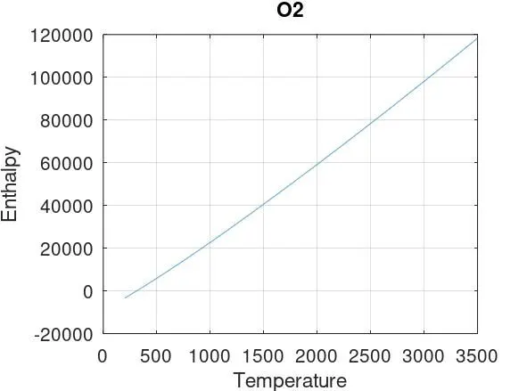
- Entropy-Temperature graph:
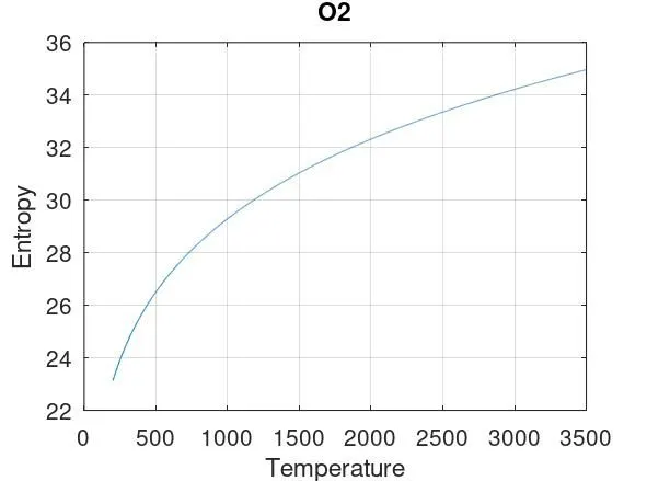
- Specific Heat-Teperature graph:
- N2(Nitrogen):
- Specific Heat-Teperature graph:
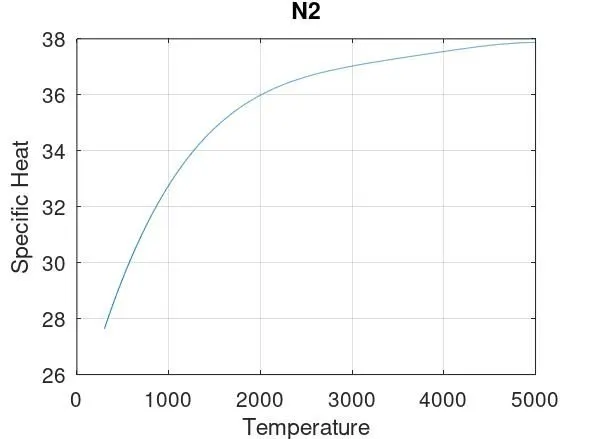
- Enthalpy-Temperature graph:
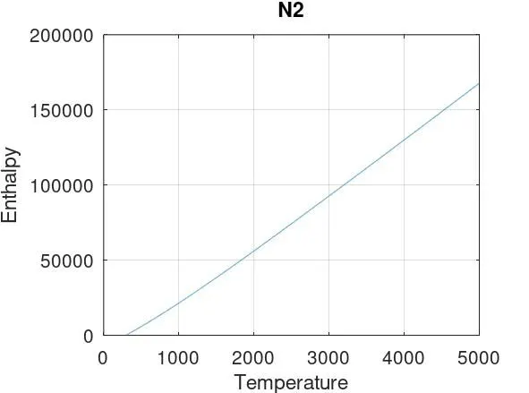
- Entropy-Temperature graph:
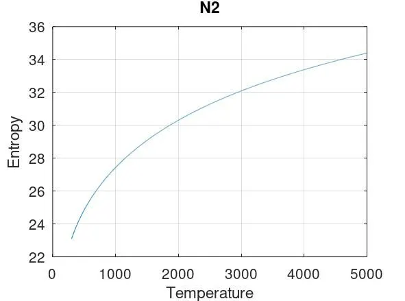
- Specific Heat-Teperature graph:
- CO2(Carbon Di-oxide):
- Specific Heat-Teperature graph:
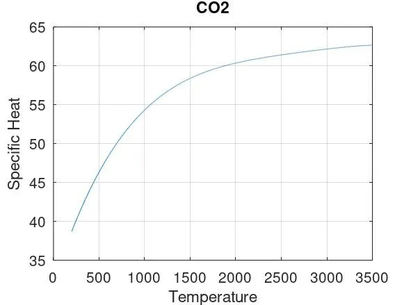
- Enthalpy-Temperature graph:
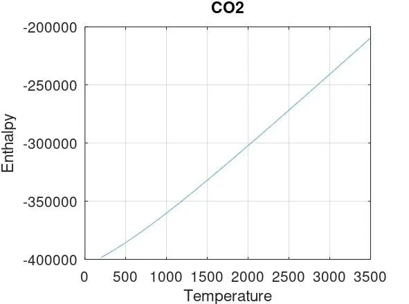
- Entropy-Temperature graph:
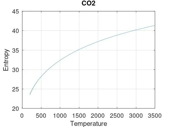
- Specific Heat-Teperature graph:
Molecular Mass:
The screenshot of the output screen.