Week 3.2 - 2R Robotic Arm Challenge

Objective:

Write a program in Matlab to simulate the forward kinematics of a 2R Robotic Arm, as shown in the video.

Create an animation file of the plot.

Input:

%program for robotic arm 2R
close all
clear all
clc

%inputs

l1=1.5;
l2=1;

theta1= linspace(0,90,19);
theta2= linspace(0,90,19);

x0 = 0;
y0 = 0;

ct = 1;

Explanation:

The inputs are defined. the arrays theta1 and theta2 is defined by the linspace() function. linspace() function gives evenly spaced elemnts from the start varible to end variable.

Syntax:

linspace(start_val,end_val,number_of_elements)

if number of elements is not defined, then the function gives '100' evenly spaced.

x0, y0 are the initial points of the first link.

l1 l2 are the lengths of first and second links.

ct is the variable introduced fir the loop counter for the gif creation

'For' loop:

Input:

%for loop

for j=1:length(theta1)
  THETA1=theta1(j);

  for k=1:length(theta2)
    THETA2=theta2(k);

    x1 = l1*cosd(THETA1);
    y1 = l1*sind(THETA1);

    x2 = x1 + l2*cosd(THETA2);
    y2 = y1 + l2*sind(THETA2);

    %plot the graphs

    %if function to create and modify gif
    ct=ct+1;


  end
end

Explanation:

Using the nested 'for' loop we can find the position of the llinks at each position.

Syntax:

for condition_1

statement_1

for condition_2

statement_2

end

end

The first 'for' loop is used for all the values of link-1 and second loop is used for all the values of link-2.

Insted of using sin() and cos(), we have used sind() and cosd() functions because in sin() & cos(), the functions consider the inputs in 'Radians'

sind() & cosd() function considers the inputs in degrees.

THETA1 and THETA2 are angles in the arrays theta1 and theta 2

Plot the graphs:

Input:

    %plot the graphs

    t_1 = sprintf("Theta1= %d \n",THETA1);
    t_2 = sprintf("Theta2= %d",THETA2);
    t_full = strcat(t_1,t_2);



    plot([x0 x1],[y0 y1],'linewidth',4,'color','r',[x1 x2],[y1 y2],'linewidth',3,'color','b');
    title(t_full);
    axis([-0.2 3.5 -0.2 3.5]);
    pause(0.01);

    frame = getframe(gcf);
    im = frame2im(frame);
    

Explanation:

The graph is plotted using the plot() funtion. The syntax used is

plot([x_start x_end], [y_start y_end], 'linewidth',linewidth_value,'color','color_alphabet')

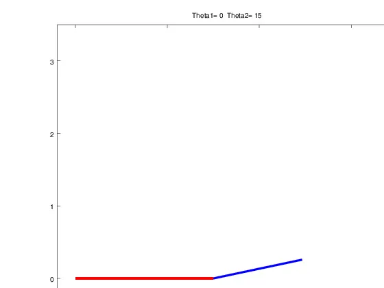
for clear understanding, We used the title to display the values of theta1 and theta2.We used sprintf() & strcat() functions to crate the title string

sprintf("string"Value to be in string)

%d takes the interger value

'/n' adds a new line

strcat(string_1 + string_2) concatenates two or more strings horizontally.

Then we add the title to the graph the syntax is:

title(title string)

we have to fix the axis to keep the frames constant for the video the syntax is:

axis([x_start x_end y_start y_end])

pause() function pauses the graph from gointo another graph the syntax is

pause(time_limit)

Animation is a collection of several images. so we need to save each and every plot. So, we use the getframe() function to save the plot as a frame.

frame = getframe(gcf)

here gcf lists all the properties of the frame.

now the frame have to be converted into image to create the gif. for that, we use frame2in() function. The frame2im() function returns RGB image

im = frame2im(frame)

'if' function for gif creation:

Input:

    if ct == 1;
          % Create GIF file
          imwrite(im,'animation-2.gif','gif','DelayTime', 0.01, 'Compression' , 'lzw');
      else
          % Add each new plot to GIF
          imwrite(im,'animation-2.gif','gif','WriteMode','append','DelayTime', 0.01 , 'Compression' , 'lzw');
      end

Explanation:

First we have to create a gif file and constantly add new images to the newly created gif file. For that we use, if loop the syntax is:

if condition

statement_1-------------------->if condition is true

else

statement_2-------------------->if condition is false

end

Here the ct is used as the variable for the gif file. at ct=1 we create the gif file and the afterwards we keep adding the images to the gif fife.

To create the gif file we use, the imwrite() function. imwrite() function returns the input image into required filetype. the syntax is:

For creating: imwrite(image_input,filename_string, filetype,'Delay time',delay time value,'compression',compression type)

For modifying: imwrite(image_input,filename_string, filetype,'writemode','append','Delay time',delay time value,'compression',compression type)

Image input is the current plot.

filename is animation-2.gif

file type gif

Delay time is 0.01 sec

compression type is lzw. LZW is A lossless compression type that supports multiple bit depths.

Output:

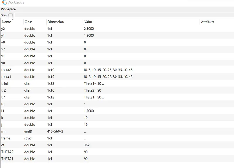
Workspace:

Errors faced:

1. imwrite() did not take the saved frame

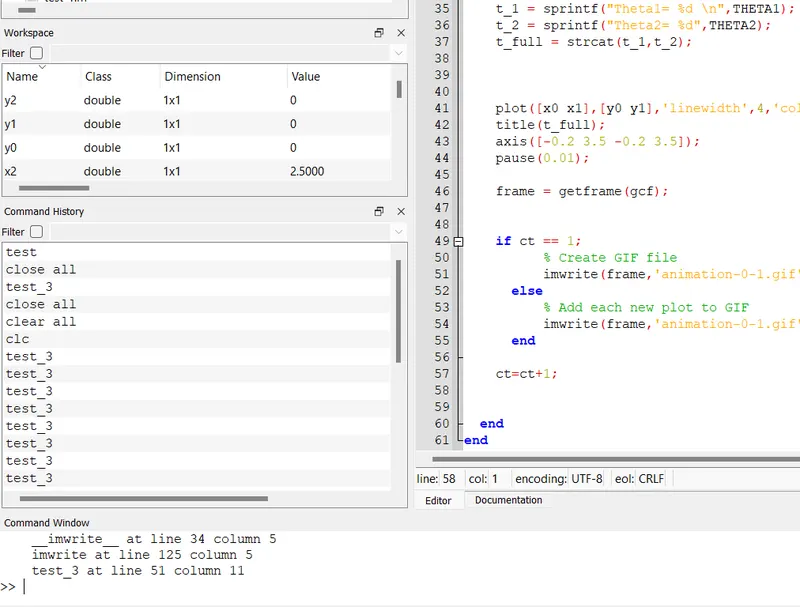
Solution:

I coverted the frame into image file using the frame2im() function.

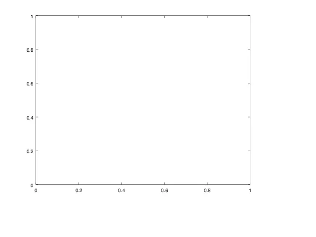
2. Octave4.0.0 was not working smoothly

The frames wre not uniform even thoughaxis was fixed. Sometimes the frame gives a blank image or a blank graph in middle. Some times the graph itself was incomplete.

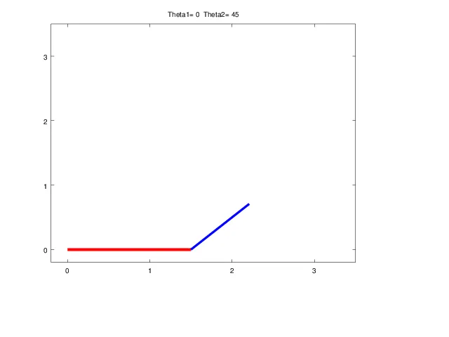
Solution:

I updated the Octave softawre to from 4.0.0 to 7.2.0