Week 5 - Curve fitting
1. What does popt and pcov mean? (Watch the video to get some context)
Ans:
Popt (Optimal parameters) :
This is an array containing the best-fit values of the parameters for your curve-fitting function. Example: If your function is f(t)=a⋅t^2+b⋅t+cf(t)=a⋅t2+b⋅t+c, popt will return the best-fit values for a, b, and c.
pcov (Covariance Matrix) :
This matrix gives an estimate of the uncertainty in the parameters. Diagonal elements represent the variances of the parameters. The off-diagonal elements represent the covariance between pairs of parameters, which shows how changes in one parameter might affect another.
2. What does np.array(temperature) do?
Ans: Ans:
Converts the list into arrays of temperature
3.3. What does the * in *popt mean?
Ans:
the "*" operator ensures the data is unpacked and passed as individual elements instead of passing it as a whole
Example:
If popt = [2, 3, 4] and func(t, a, b, c) is the
function, func(np.array(temperature), *popt) is equivalent to func(temperature,a=2,b=3,c=4)
4. Write code to fit a linear and cubic polynomial for the Cp data. Explain if your results are good or bad.
Ans:
def cubic_func(t, a, b, c, d):
return a * np.power(t, 3) + b * np.power(t, 2) + c * t + d
# Reading thermodynamic data from a file
def read_file():
temperature = []
cp = []
with open('data.txt', 'r') as file:
for line in file:
values = line.split(',')
temperature.append(float(values[0]))
cp.append(float(values[1]))
return temperature, cp
# Main program
temperature, cp = read_file()
# Perform curve fitting for linear and cubic functions
popt_linear, pcov_linear = curve_fit(linear_func, temperature, cp)
popt_cubic, pcov_cubic = curve_fit(cubic_func, temperature, cp)
# Generate fitted Cp values for both models
fit_cp_linear = linear_func(np.array(temperature), *popt_linear)
fit_cp_cubic = cubic_func(np.array(temperature), *popt_cubic)
# Plot actual data and both fits
plt.plot(temperature, cp, 'o',, label='Actual Data')
plt.plot(temperature, fit_cp_linear,, linewidth=2, label='Linear Fit')
plt.plot(temperature, fit_cp_cubic,, linewidth=2, label='Cubic Fit')
plt.legend()
plt.xlabel('Temperature [K]')
plt.ylabel('Cp')
plt.title('Linear vs Cubic Polynomial Fit')
plt.grid(True)
plt.show()
Output:
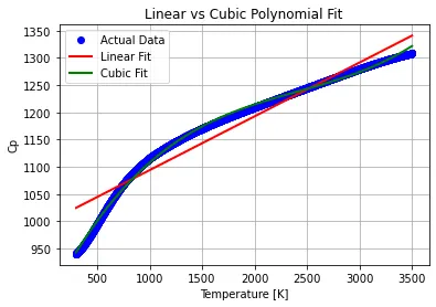
We can see that while doing the fitting with linear fit we are not able to get a proper fit as there is multiple lapses here and there and the curve is more of a linear pattern.
Now coming to cubic fit we can see the fit is more perfect than the initial case and we can see very minimal lapses.
5. What needs to be done in order to make the curve fit perfect?
Ans:
1) Use higher-order polynomials or functions tailored to the physical phenomenon (e.g., exponential, logarithmic).
2) Remove outliers or noisy data points.
3) If certain data points are more reliable, use weighted curve fitting to give them higher importance.
4) Ensure the dataset full behavior is captured
6. Show empirically as to how well your curve has been fit.
Ans:
For checking the fitness we use R2 method. This shows level of the variability in the data is captured by the model.
(Note: this program cannot run seperateley, need to run with the main program)
#checking the fitness
# Calculate R-squared for cubic fit
residuals = cp - fit_cp_cubic
ss_res = np.sum(residuals**2) # Sum of squared residuals
ss_tot = np.sum((cp - np.mean(cp))**2) # Total sum of squares
r_squared = 1 - (ss_res / ss_tot)
print("R-squared for Cubic Fit:", r_squared)
Output: R-squared for Cubic Fit: 0.9967259467140538
This shows our fit is near to perfect.