Week 4.1 - Genetic Algorithm

Pogram to optimise the stalagmite function and find the global maxima of the function

Optimization: Optimization deals with how to minimize or maximize a function which deals with multiple parametetrs

Stalagmite function: mathematical function used to generate local maximas and minimas

local maximas-large peaks in graph

local minima- small peaks in graph

ga (genetic algorithm)- inbuilt function which returns minimum value of the peaknote

note: we have given a -ve sighn to function so that ga return local maximas

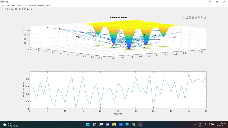
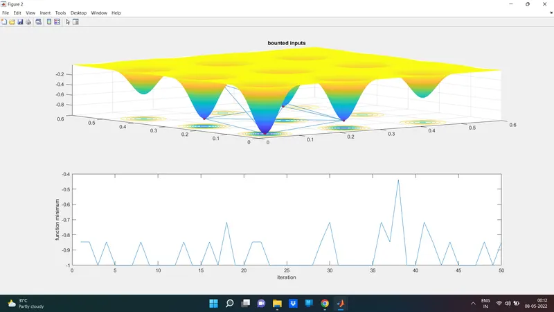
Each and every time ga gives different outputs so we are doing 3 case studies with 50 iterations

In case 1: ga predicts 50 minimas most of it are out of surge space

case 2: we have given upper and lower bound so that maxima prediction is consrained within the boundary

case 3: we keeping the same boundary condition and increasing the population size

MATLAB PROGRAM

clear all
close all
clc
%defining space
x=linspace(0,0.6,150);
y=linspace(0,0.6,150);
%creating 2D mesh
[xx yy]=meshgrid(x,y);
%evaluating stalagmate function
for i=1:length(xx)
    for j=1:length(yy)
        input_vector(1)=xx(i,j);
        input_vector(2)=yy(i,j);
        %stalagmate takes in input 
        f(i,j)=stalagmite_func(input_vector);
    end
end

%doing 50 studies for 3 cases and creating subplot for all to visualize
%further
numof_study=50;

%GA STUDY CASE 1

tic
for i=1:numof_study
   [inputs,fopt(i)]=ga(@stalagmite_func, 2);
xopt(i)=inputs(1);
yopt(i)=inputs(2);
end
%determining study time
study1time=toc
figure(1)
subplot(2,1,1)
%creating 3D plot 
surfc(x,y,f)
shading interp
hold on
% plot3 command is used for creating a 3D point or line plot
plot3(xopt,yopt,fopt,'marker','o','MarkerSize',5,'MarkerFaceColor','r')
title('unbounted inputs')
subplot(2,1,2)
plot(fopt)
xlabel('iteration')
ylabel('function minimum')

%GA STUDY CASE 2 with upper and lower bounds

tic
for i=1:numof_study
    [inputs,fopt(i)]=ga(@stalagmite_func,2,[],[],[],[],[0;0],[1;1]);
    xopt(i)=inputs(1);
     yopt(i)=inputs(2);
end
%determining study time
study2time=toc

figure(2)
subplot(2,1,1)
%creating 3D plot 
surfc(x,y,f)
shading interp
hold on
% plot3 command is used for creating a 3D point or line plot
plot3(xopt,yopt,fopt,'marker','o','MarkerSize',5,'MarkerFaceColor','r')
title('bounted inputs')
subplot(2,1,2)
plot(fopt)
xlabel('iteration')
ylabel('function minimum')

%STUDY CASE 3 INCREASING GA ITERATIONS BY INCREASING THE POPULATION SIZE
%by default population size is 50

tic
%by default population size is 50 using option syntax we are able to
%increase the population size
options=optimoptions('ga');
options=optimoptions(options,'PopulationSize',300);
tic
for i=1:numof_study
   
   %since we have used options syntax to increase the polpulation size we
   %ise ga syntax with options in it
     [inputs, fopt(i)] =  ga(@stalagmite_func,2,[],[],[],[],[0:0],[1:1], [],[],options); 
    xopt(i)=inputs(1);
     yopt(i)=inputs(2);
end
%determining study time
study3time=toc

figure(3)
subplot(2,1,1)
%creating 3D plot 
surfc(x,y,f)
shading interp
hold on
% plot3 command is used for creating a 3D point or line plot
plot3(xopt,yopt,fopt,'marker','o','MarkerSize',5,'MarkerFaceColor','r')
title('bounted inputs with modified population size')
subplot(2,1,2)
plot(fopt)
xlabel('iteration')
ylabel('function minimum')

MATLAB FUNCTION

function [z]=stalagmite_func(input_vector)
%we pass two values for input vectors here
x=input_vector(1);
y=input_vector(2);
%based on the main eqn we have written the below codes 
f1x=(sin(5.1*pi*x+0.5))^6;
f1y=(sin(5.1*pi*y+0.5))^6;
f2x=exp(-4*log(2)*((x-0.0667)^2)/0.64);
f2y=exp(-4*log(2)*((y-0.0667)^2)/0.64);
%negative sighn has been given because ga returns inputs where the function
%is minimun but we want the max value
z=-f1x*f1y*f2x*f2y;
end

OUTPUTS

CASE1:

CASE 2:

CASE 3:

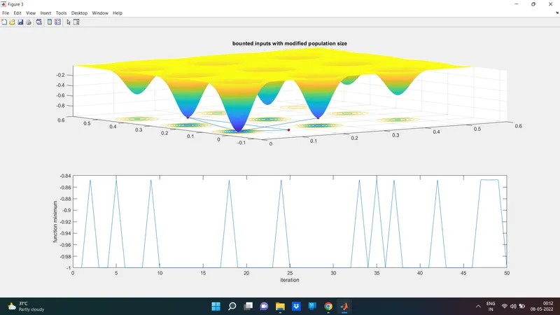
INFERENCE:

During 1st case during 50 iterations most of the values were out of surge space so to overcome this we added upper and lowe bound to constrain he points between a specific value. so we get a much better plot, still we can see ga have predicted even the lower peaks as maxima. so to overcome this we have added population size, by default it uses 50 as population size. By increasing the population size to 300 we are better able to predict the maximas as seen in case 3

REFERENCE:

Matlab documentation for GA and its syntax

https://in.mathworks.com/help/gads/ga.html

https://in.mathworks.com/help/optim/ug/optim.problemdef.optimizationproblem.optimoptions.html