Week 5 - Curve fitting
Answers:
1. What does popt and pcov mean? (Watch the video to get some context)
popt and pcov are the results of the curve_fit function used to calculate the approximate curve we want to tend the actual noisy data to.
popt contains the optimized parameters or the best fit values.
pcov contains the covariance of parameters (the measure of accuracy or fit)
2. What does np.array(temperature) do?
temperature read from file using open(), is raw data. it could be a list of values or other type of data structure. when we use np.array(temperature), the resultant value is converted into a numpy.ndarray, which supports a variety of powerful mathematical and array operations.
3. What does the * in *popt mean?
*popt is the key part.
popt is a list or array containing the optimized parameters (the best-fitting values for the model). The * is the unpacking operator in Python, which unpacks the values from popt and passes them as individual arguments to the model function.
for example, in the code, on line
fit_cp = func(np.array(temperature), *pOpt)
the pOpt is the calculated values of new Cp via the curve_fit function. plotting these values overlapping the original cp values on graph, will give us the required curve_fit comparison, whether the cureve fit is good enough or not.
4. Write code to fit a linear and cubic polynomial for the Cp data. Explain if your results are good or bad.
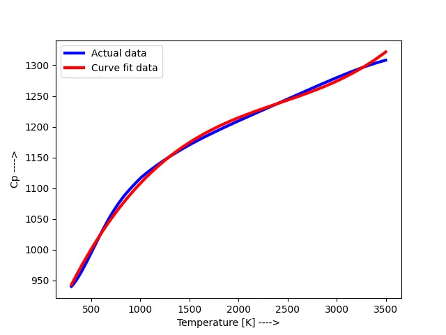
to fit a cubic polynomial:
code:
import numpy as np
import matplotlib.pyplot as plt
from scipy.optimize import curve_fit
# this is a Python program to do a curve fir on existing thermodynamic data
#curveFit function
# a, b, and c are the parameters that we want to estimate using curve_fit.
#t is the independent variable - temperature.
def func(t, a, b, c, d):
return a * pow(t, 3) + b * pow(t, 2) + c * t + d
#read thermodynamic data file
def read_file():
temperature = []
cp = []
for line in open('data', 'r'):
values = line.split(',')
temperature.append(float(values[0]))
cp.append(float(values[1]))
return [temperature, cp]
#main program
temperature, cp = read_file()
pOpt, pCov = curve_fit(func, temperature, cp)
fit_cp = func(np.array(temperature), *pOpt)
print(pCov)
#plots
plt.plot(temperature, cp, color = 'blue', linewidth = 3)
plt.plot(temperature, fit_cp, color = 'red', linewidth = 3)
plt.legend(['Actual data', 'Curve fit data'])
plt.xlabel('Temperature [K] ---->')
plt.ylabel('Cp ---->')
plt.show()
pCOv of the above cure-fit is as follows:
[[ 2.40372527e-20 -1.36976286e-16 2.23265241e-13 -9.46095475e-11]
[-1.36976286e-16 7.96382734e-13 -1.33238995e-09 5.82722196e-07]
[ 2.23265241e-13 -1.33238995e-09 2.31292603e-06 -1.06487773e-03]
[-9.46095475e-11 5.82722196e-07 -1.06487773e-03 5.40651123e-01]]
The uncertainty in the parameter a is sqrt(2.40372527e-20) = 1.5503951980059792e-10
The uncertainty in the parameter b is sqrt(7.96382734e-13) = 8.924027868625243e-07
The uncertainty in the parameter c is sqrt(2.31292603e-06) = 0.0015208307039246676
The uncertainty in the parameter d is sqrt(5.40651123e-01) = 0.7352898224509843
as we see:
the values along the diagonal are very less. this means the variance int he values of a, b, c and d variables is very less.
all other values are also on lower side which means that the co-variance of a w.r.t b is negligible which is better for a curve-fit result.
the plot is as below:
to fit a linear polynomial:
code:
import numpy as np
import matplotlib.pyplot as plt
from scipy.optimize import curve_fit
# this is a Python program to do a curve fir on existing thermodynamic data
#curveFit function
# a, b, and c are the parameters that we want to estimate using curve_fit.
#t is the independent variable - temperature.
def func(t, a, b):
return a * t + b
#read thermodynamic data file
def read_file():
temperature = []
cp = []
for line in open('data', 'r'):
values = line.split(',')
temperature.append(float(values[0]))
cp.append(float(values[1]))
return [temperature, cp]
#main program
temperature, cp = read_file()
pOpt, pCov = curve_fit(func, temperature, cp)
fit_cp = func(np.array(temperature), *pOpt)
print(pCov)
#plots
plt.plot(temperature, cp, color = 'blue', linewidth = 3)
plt.plot(temperature, fit_cp, color = 'red', linewidth = 3)
plt.legend(['Actual data', 'Curve fit data'])
plt.xlabel('Temperature [K] ---->')
plt.ylabel('Cp ---->')
plt.show()
pCOv of the above cure-fit is as follows:
[[ 2.47696157e-07 -4.70498850e-04]
[-4.70498850e-04 1.10507993e+00]]
The uncertainty in the parameter a is sqrt(2.47696157e-07) = 0.0004976908247094776
The uncertainty in the parameter b is sqrt(1.10507993e+00) = 1.051227820217863
as wee see,
the diagonal values are significantly greater in this case than the former one. this implies that the variance of variables a and b is much greater and the curve-fit result are not very convincing.
other values except diagonal left - right are also significantly greater in this case than the former one. so the co-varince is also a problem here.
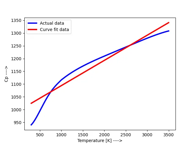
clearly, the cubic polynomial curve-fit is better in approximation of the actual noisy data collected from file.
5. What needs to be done in order to make the curve fit perfect?
in order to make the curve fit perfect, we need to have a higher order polynomial into the model. this statement is corroborated by the answer and findings for the previous question.
if this is also a not so good fit, then we can try to split the graph into separate parts and have different polynomial approximations/models for different parts of the graphs, which when joined will be a better curve-fit result.
6. Show empirically as to how well your curve has been fit.
i tried with quadratic polynomial as well.
here is the graph:
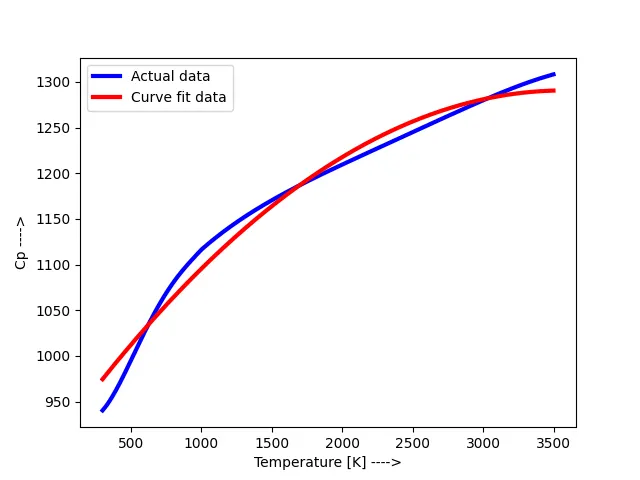
pCov values for the above graph are:
[[ 9.06275935e-14 -3.44294227e-10 2.49657904e-07]
[-3.44294227e-10 1.36984217e-06 -1.06596942e-03]
[ 2.49657904e-07 -1.06596942e-03 9.63771165e-01]]
these values are better than that of linear and bad than that of cubic approximation model.
The uncertainty in the parameter a is sqrt(9.06275935e-14) = 3.010441720080294e-07
The uncertainty in the parameter b is sqrt(1.36984217e-06) = 0.0011704025674954752
The uncertainty in the parameter c is sqrt(9.63771165e-01) = 0.9817184754296926