Project 1 - Parsing NASA thermodynamic data
The function that extracts the 14 co-efficients and calculates the enthalpy, entropy and specific heats is written.
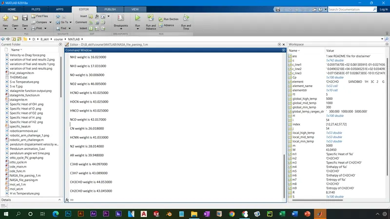
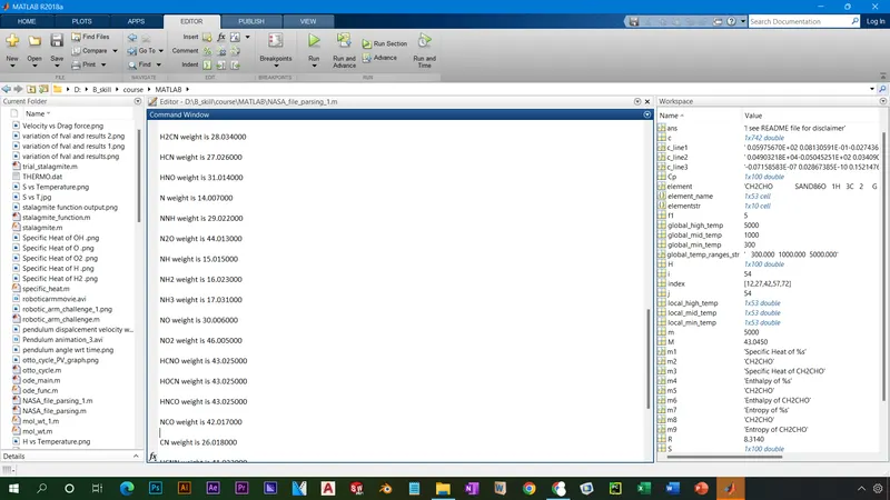
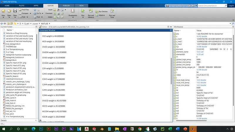
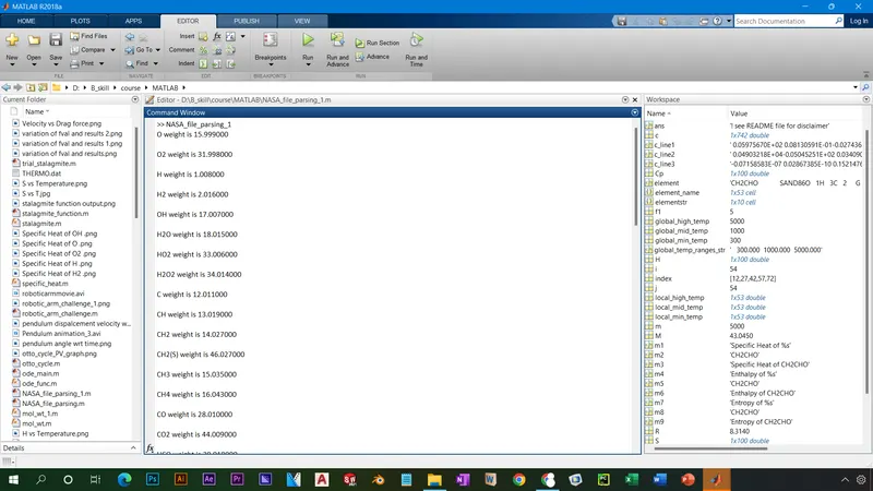
Molecular weight of each species is calculated an displayed in the command window.
Plot of Cp, Enthalpy and Entropy for the local temperature range (low temperature : high temperature) specific for each species is also drawn.
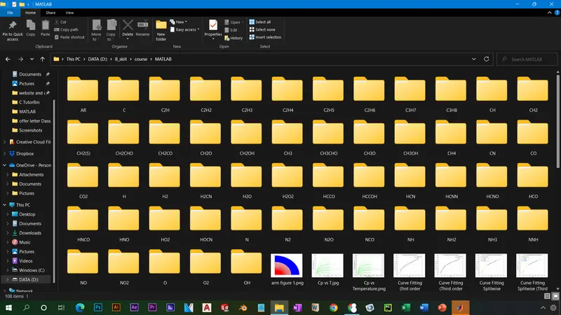
Saved the plots as images with appropriate names and dumped them in separate folders for each species with suitable name. All these were generated automatically.
The following is the code and description:
The main code:
% NASA file parsing

f1 = fopen('THERMO.dat', 'r'); % open file
title = fgetl(f1); % get the title of file
global_temp_ranges_str = fgetl(f1); % read the global temperature ranges
splitt = strsplit(global_temp_ranges_str, ' '); % split the temperatures
for i = 2:4
    str_temp(i) = str2num( splitt {:,i} ); % store the temperatures
end
global_min_temp = str_temp(2); % name the min temp
global_mid_temp = str_temp(3); % name the mid temp
global_high_temp = str_temp(4); % name the high temp
fgetl(f1); % read the next line (no use)
fgetl(f1); % read the next line (no use)
fgetl(f1); % read the next line (no use)
% header reading is finished

% actual data reading starts

    for i = 1:53

    element = fgetl(f1); % read the first line of first element
    elementstr = strsplit(element, ' '); % split the line
    element_name(i) = elementstr(:,1); % store the element name
    local_min_temp(i) = str2num(elementstr{:,end - 3}); % store the local min temp
    local_high_temp(i) = str2num(elementstr{:,end - 2}); % store the local mid temp
    local_mid_temp(i) = str2num(elementstr{:,end - 1}); % store the local high temp

    c_line1 = fgetl(f1); % read the first coefficient line
    index = strfind(c_line1, 'E'); % split the line by 'E' and get the place values of 'E'
    c(i * 14 - 13) = str2num(c_line1(1:index(1)+3)); % store the number
    c(i * 14 - 12) = str2num(c_line1(index(1)+4:index(2)+3)); % store the number
    c(i * 14 - 11) = str2num(c_line1(index(2)+4:index(3)+3)); % store the number
    c(i * 14 - 10) = str2num(c_line1(index(3)+4:index(4)+3)); % store the number
    c(i * 14 - 9) = str2num(c_line1(index(4)+4:index(5)+3)); % store the number

    c_line2 = fgetl(f1); % read the second coefficient line
    c(i * 14 - 8) = str2num(c_line2(1:index(1)+3)); % store the number
    c(i * 14 - 7) = str2num(c_line2(index(1)+4:index(2)+3)); % store the number
    c(i * 14 - 6) = str2num(c_line2(index(2)+4:index(3)+3)); % store the number
    c(i * 14 - 5) = str2num(c_line2(index(3)+4:index(4)+3)); % store the number
    c(i * 14 - 4) = str2num(c_line2(index(4)+4:index(5)+3)); % store the number

    c_line3 = fgetl(f1); % read the third coefficient line
    c(i * 14 - 3) = str2num(c_line3(1:index(1)+3)); % store the number
    c(i * 14 - 2) = str2num(c_line3(index(1)+4:index(2)+3)); % store the number
    c(i * 14 - 1) = str2num(c_line3(index(2)+4:index(3)+3)); % store the number
    c(i * 14 - 0) = str2num(c_line3(index(3)+4:index(4)+3)); % store the number

    i = i + 1;
    end
% L = char(element_name);
    R = 8.314; % universal gas constant

    for j = 1:53 % to plot the graphs of all 53 species
        mkdir(['D:\B_skill\course\MATLAB\ ', char(element_name(j))]) % a directory is made in the specified location
        cd(sprintf('D:/B_skill/course/MATLAB/ %s ', char(element_name(j)))) % folders of the element_name are made

        t = linspace(local_min_temp(j), local_high_temp(j), 100); % for x-axis of graph
        for m = local_min_temp(j):local_high_temp(j) % range for the x-axis of graph is specified
            if m < local_mid_temp(j) % formulas written
                    Cp = R * (c(j * 14 - 6) + c(j * 14 - 5).*t + c(j * 14 - 4)*(t).^2 + c(j * 14 - 3)*(t).^3 + c(j * 14 - 2)*(t).^4);
                    H = R .* t .* (c(j * 14 - 6) + ((c(j * 14 - 5))/2).*t + ((c(j * 14 - 4))/3).*(t).^2 + ((c(j * 14 - 3))/4).*(t).^3 + ((c(j * 14 - 2))/5).*(t).^4 + (c(j * 14 - 1))./t);
                    S = R * (c(j * 14 - 6) * log(t) + c(j * 14 - 5) .* t + ((c(j * 14 - 4))/2) .* (t).^2 + ((c(j * 14 - 3))/3) .* (t).^3 + ((c(j * 14 - 2))/4) .* (t).^4 + c(j * 14 - 0));
            else
                Cp = R * (c(j * 14 - 13) + c(j * 14 - 12).*t + c(j * 14 - 11)*(t).^2 + c(j * 14 - 10)*(t).^3 + c(j * 14 - 9)*(t).^4);
                H = R .* t .* (c(j * 14 - 13) + ((c(j * 14 - 12))/2).*t + ((c(j * 14 - 11))/3).*(t).^2 + ((c(j * 14 - 10))/4).*(t).^3 + ((c(j * 14 - 9))/5).*(t).^4 + (c(j * 14 - 8))./t);
                S = R * (c(j * 14 - 13) * log(t) + c(j * 14 - 12) .* t + ((c(j * 14 - 11))/2) .* (t).^2 + ((c(j * 14 - 10))/3) .* (t).^3 + ((c(j * 14 - 9))/4) .* (t).^4 + c(j * 14 - 7));
            %m = m + ((local_high_temp(j) - local_min_temp(j))/100);
            end
        end
                figure(1)
                plot(t(1,:), Cp(1,:),'color','g');
                xlabel('Temperature (T)')
                ylabel('Specific Heat (J/Kg - K)')

                m1 = 'Specific Heat of %s'; % name to the image of the graph saved is given here
                m2 = char(element_name(j)); % name of the element specified
                m3 = sprintf(m1,m2); % m1 and m2 are combined
                saveas(figure(1),sprintf('%s .png',m3)) % figure is saved in this name format
                grid on

                figure(2)
                plot(t(1,:), H(1,:),'color','g');
                xlabel('Temperature (T)')
                ylabel('Enthalpy (J/mol)')

                m4 = 'Enthalpy of %s'; % name to the image of the graph saved is given here
                m5 = char(element_name(j)); % name of the element specified
                m6 = sprintf(m4,m5); % m1 and m2 are combined
                saveas(figure(2),sprintf('%s .png',m6)) % figure is saved in this name format
                grid on

                figure(3)
                plot(t(1,:), S(1,:),'color','g');
                xlabel('Temperature (T)')
                ylabel('Entropy (J/K)')

                m7 = 'Entropy of %s'; % name to the image of the graph saved is given here
                m8 = char(element_name(j)); % name of the element specified
                m9 = sprintf(m7,m8); % m1 and m2 are combined
                saveas(figure(3),sprintf('%s .png',m9)) % figure is saved in this name format
                grid on
                cd('D:\B_skill\course\MATLAB\') % once all the three figures are saved, we enter new folder (species)

%      molecular weight
    [M] = mol_wt_1( char(element_name(j)) ); % numerical value is processed from here
    Z = sprintf('%s weight is %f \n', char(element_name(j)), M); % output of weights is printed from here
    disp(Z) % value of Z is displayed
    j = j + 1;
    end
The function code:
% % function to calculate molecular weight of the species

function mol_wt = mol_wt_1(element_name)
%element_name = 'C3H8';
weight = 0;
elements = {'H', 'C', 'N', 'O', 'A', 'S'};
mass = [1.008, 12.011, 14.007, 15.999, 39.948, 32.000];
 for u = 1: length(element_name)
     for v = 1:length(elements)
         if strcmpi(element_name(u), elements(v))
             weight = weight + mass(v);
             y = v;
         end
     end
     number = str2double(element_name(u));
     if number > 1
         weight = weight + ( mass(y) * (number - 1) );
     end
 mol_wt = weight;
 end
end
Screenshot of the dumped files:
plots of O2:
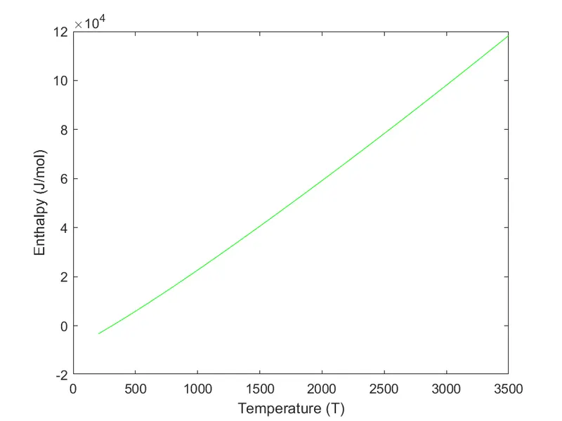
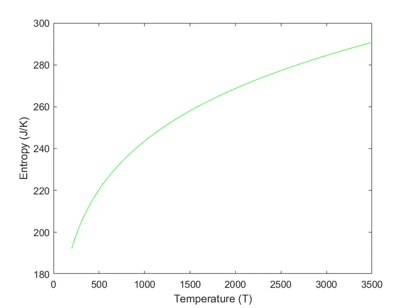
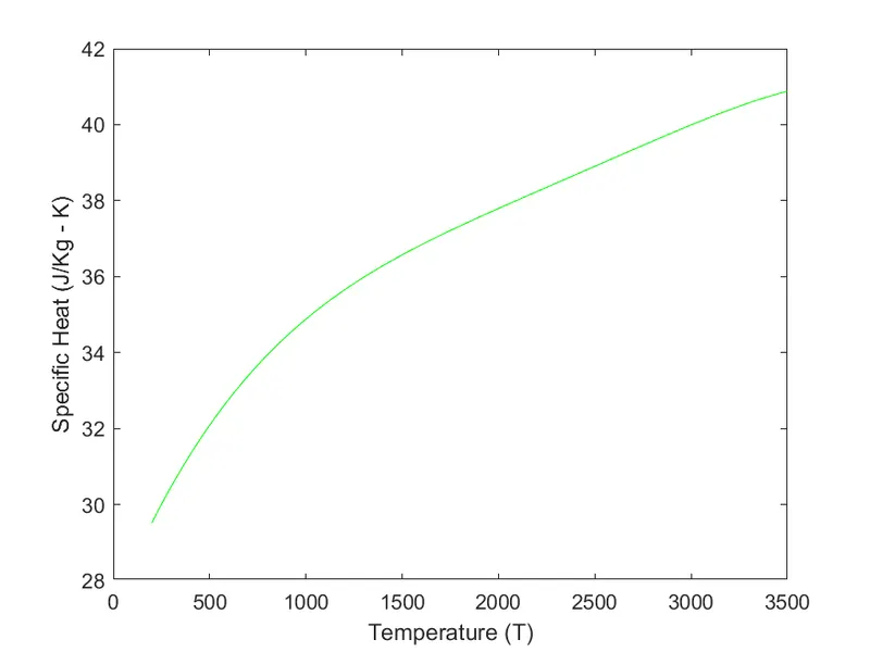
Plots of N2:
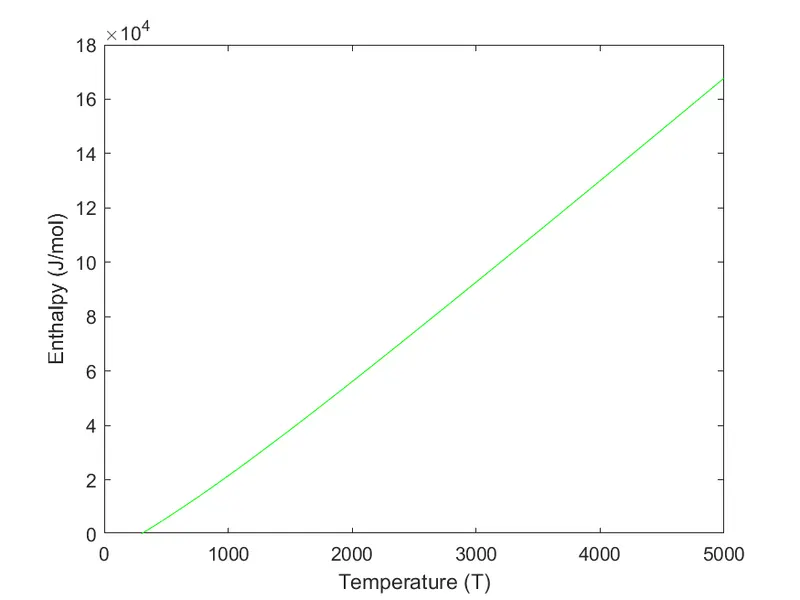
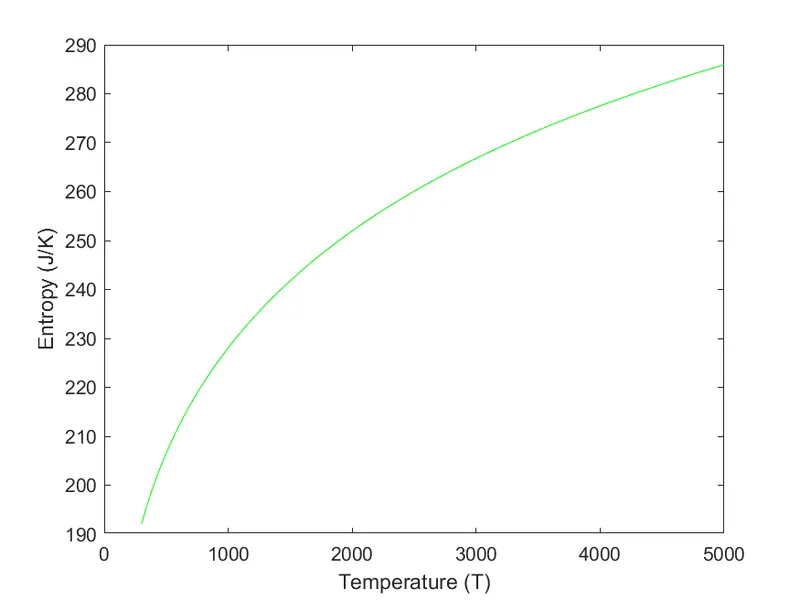
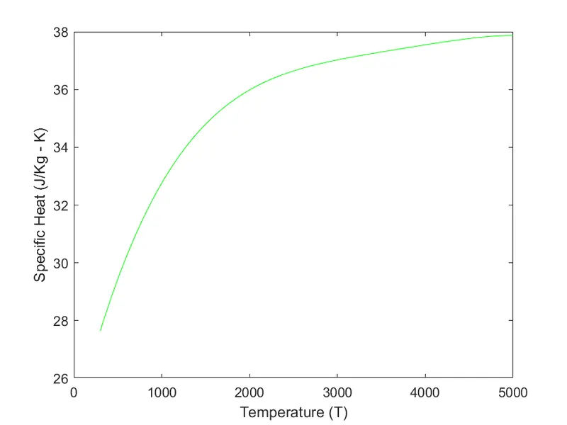
Plots of CO2:
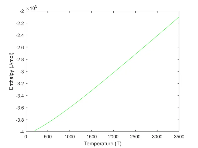
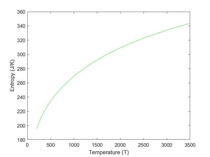
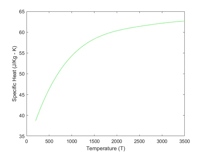
The screenshot of weights printed in the command window:
errors faced:
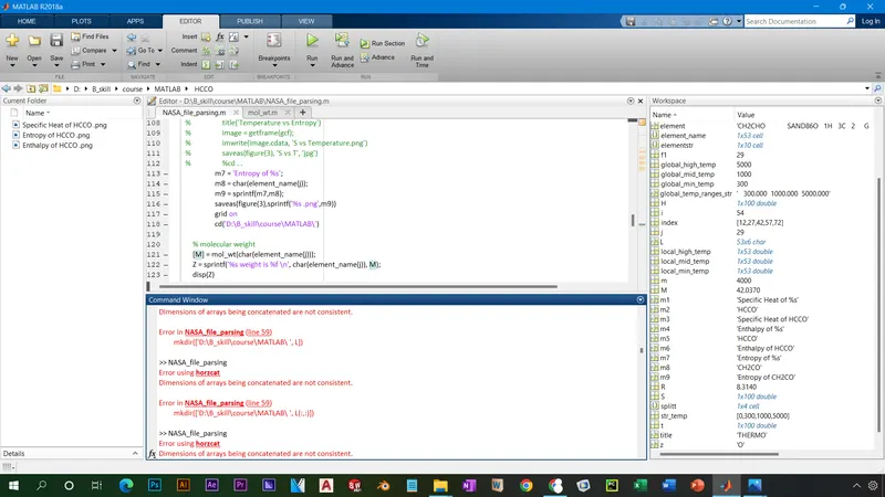
dimensions of array was re-checked.
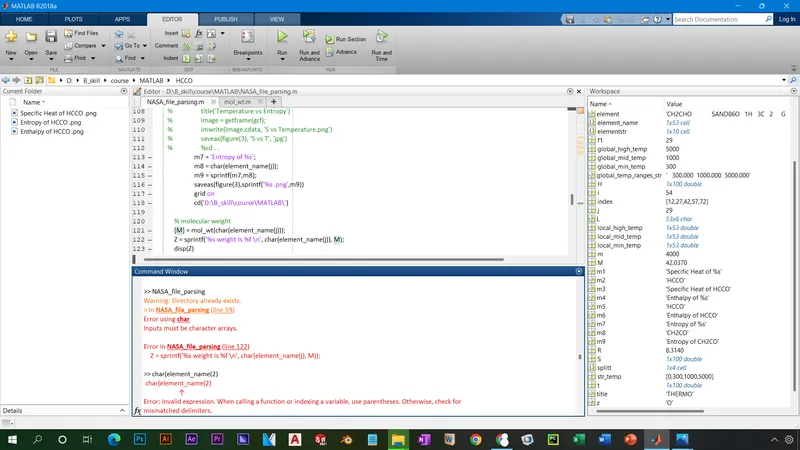
syntax error.
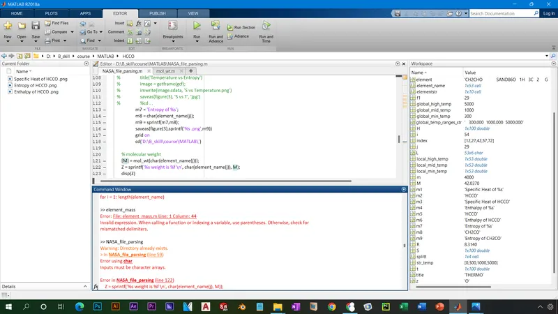
character, cell and array elements were taken care of independently to get rid of error.
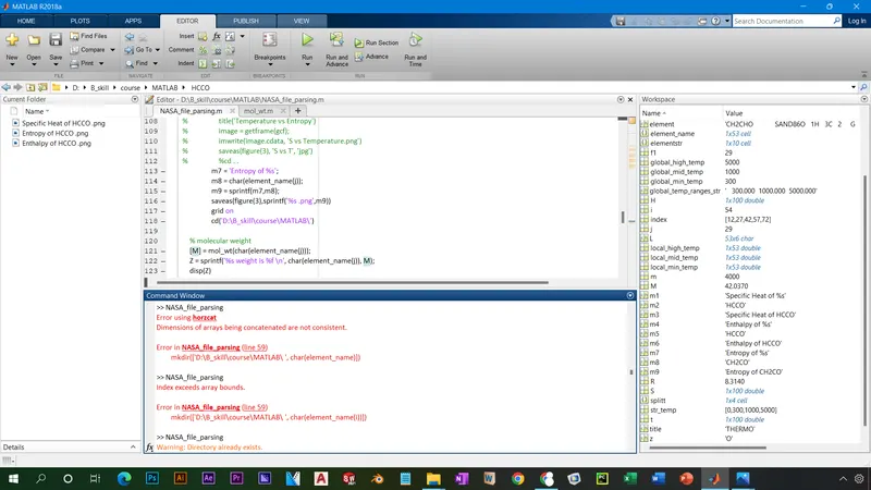
making directory syntax code was properly written after error.
cd(sprintf('D:/B_skill/course/MATLAB/ %s ', char(element_name(j)))) % folders of the element_name are made
this line was modified properly to get rid of error.
MATLAB help services was used for research of new code syntax.
logic behind choosing aspects to parse out the files:
1. the file is a repetitive information, therefore we can code it to save values appearing on repeated places.
2. strings should be converted to numbers to carry out calculations, wherever necessary.
3. function should be written correctly to calculate the mass of the species.
4. the main logic is still reading the values on repetitive places and doing all calculations necessary.