Week 5 - Curve fitting

Aim:

To write a python script to perform curve fitting from the given data and answer the following problems given below.

Objective:

1. What does popt and pcov mean? (Watch the video to get some context)

2. What does np.array(temperature) do?

3. What does the * in *popt mean?

4. Write code to fit a linear and cubic polynomial for the Cp data. Explain if your results are good or bad.

5. What needs to be done in order to make the curve fit perfect?

6. Show empirically as to how well your curve has been fit.

Solution:

1. What does popt and pcov mean? (Watch the video to get some context)

In Python, especially when utilizing the scipy.optimize.curve_fit function from the SciPylibrary, the terms "popt" and "pcov" hold specific significance:

- "popt" An abbreviation for "optimized parameters" refers to a variable that holds parameter values optimized or changed during curve fitting to data. Using the curve_fit function aligns a model with data points by fine-tuning its parameters for optimal accuracy. The "popt" variable contains the refined parameter values. In final, it is an array which contains the value of a, b, c, d, e, f, g, h, i, j.

- "pcov" "Parameter covariance" refers to a variable that stores the covariance matrix associated with improved parameter estimations. The covariance matrix provides insights into the uncertainty and linkages between parameter estimates. The diagonal members of the matrix represent parameter variances, whereas the off-diagonal components represent parameter covariance.

2. What does np.array(temperature) do?

The function 'np.array(temperature)' creates a NumPy array from the 'temperature' variable. NumPy is a powerful Python library that supports arrays, matrices, and various mathematical operations.

Using 'np.array(temperature)' transforms a list or tuple containing numeric values into a NumPy array. This transformation is helpful since arrays offer more capabilities than traditional Python lists. The benefits include optimized math computations, efficient memory consumption, and convenient element-wise operations.

3. What does the * in *popt mean?

The asterisk * in Python has different meanings based on the context. *popt separates elements in a list or tuple into distinct arguments.

Within the domain of curve fitting and function invocations, particularly when handling the scipy.optimize.curve_fit function provided by the SciPy library, the expression *popt is frequently employed to break down the contents of the popt array into individual arguments. This practice is often utilized when transmitting optimized parameters to a function that anticipates separate parameter values as its arguments.

4. Write code to fit a linear and cubic polynomial for the Cp data. Explain if your results are good or bad.

Program:

"""
Aksharat Jain
"""

import numpy as np 
import matplotlib.pyplot as plt
from scipy.optimize import curve_fit

# Define polynomial function with parameters a, b, ..., j
def f(t, a, b, c, d, e, f, g, h, i, j):
    # Depending on the degree of polynomial (I), construct the equation
    if I == 1:
        return a*t**1 + b*t**0 +   0*(c*t**7 + d*t**6 + e*t**5 + f*t**4 + g*t**3 + h*t**2 + i*t**1 + j*t**0)
    if I==2: # Algebraic Equation of Second Degree or Quadratic Equation
        return a*t**2 + b*t**1 + c*t**0 +   0*(d*t**6 + e*t**5 + f*t**4 + g*t**3 + h*t**2 + i*t**1 + j*t**0)
    if I==3: # Algebraic Equation of Third Degree or Cubic Equation
        return a*t**3 + b*t**2 + c*t**1 + d*t**0 +   0*(e*t**5 + f*t**4 + g*t**3 + h*t**2 + i*t**1 + j*t**0)
    if I==4: # Algebraic Equation of Fourth Degree
        return a*t**4 + b*t**3 + c*t**2 + d*t**1 + e*t**0 +   0*(f*t**4 + g*t**3 + h*t**2 + i*t**1 + j*t**0)
    if I==5: # Algebraic Equation of Fifth Degree 
        return a*t**5 + b*t**4 + c*t**3 + d*t**2 + e*t**1 + f*t**0 +   0*(g*t**3 + h*t**2 + i*t**1 + j*t**0)
    if I==6: # Algebraic Equation of Sixth Degree
        return a*t**6 + b*t**5 + c*t**4 + d*t**3 + e*t**2 + f*t**1 + g*t**0 +   0*(h*t**2 + i*t**1 + j*t**0)
    if I==7: # Algebraic Equation of Seventh Degree
        return a*t**7 + b*t**6 + c*t**5 + d*t**4 + e*t**3 + f*t**2 + g*t**1 + h*t**0 +   0*(i*t**1 + j*t**0)			
    if I==8: # Algebraic Equation of Eighth Degree
        return a*t**8 + b*t**7 + c*t**6 + d*t**5 + e*t**4 + f*t**3 + g*t**2 + h*t**1 + i*t**0 +   0*(j*t**0)
    if I==9: # Algebraic Equation of Ninth Degree
        return a*t**9 + b*t**8 + c*t**7 + d*t**6 + e*t**5 + f*t**4 + g*t**3 + h*t**2 + i*t**1 + j*t**0

# Function to read data from a file
def rf():
    T = []
    cp = []
    for line in open('data', 'r'):
        v = line.split(',')
        T.append(float(v[0]))
        cp.append(float(v[1]))
    return np.array(T), np.array(cp)

# Loop through polynomial degrees from 1 to 9
for I in range(1, 10):
    # Read data from file
    T, cp = rf()

    # Perform curve fitting using the defined polynomial function
    P, _ = curve_fit(f, T, cp)
    fit = f(T, *P)

    # Calculate residuals
    residuals = cp - fit

    # Calculate SSE, SSR, SST, R_squared
    SSE = np.sum(residuals**2)
    SSR = np.sum((fit - np.mean(cp))**2)
    SST = SSE + SSR
    R_squared = SSR / SST

    # Counter to keep track of plot numbers
    plot_counter = 1
    
    # Plot the actual data, the fitted curve, and residuals
    plt.plot(T, cp, color='blue', label='Actual Data')
    plt.plot(T, fit, color='orange', label='Fitted Curve')
    plt.title('Polynomial of Degree ' + str(I) + '\nSpecific Heats (Cp) vs Temperature (K)')
    plt.xlabel('Temperature (K)')
    plt.ylabel('Cp')
    plt.legend()
    plt.tight_layout()
    
    # Save the plot
    plt.savefig('plot_' + str(I) + '_data_fit.png')
    
    # Increment the plot counter
    plot_counter += 1
    
    # Display plot
    plt.show()

    # Plot residuals
    plt.plot(T, residuals, color='red', label='Residuals')
    plt.axhline(y=0, color='gray', linestyle='--')
    plt.title('Polynomial of Degree ' + str(I) + '\nResiduals vs Temperature (K)')
    plt.xlabel('Temperature (K)')
    plt.ylabel('Residuals')
    plt.legend()
    plt.tight_layout()
    
    # Save the plot
    plt.savefig('plot_' + str(I) + '_residuals.png')
    
    # Increment the plot counter
    plot_counter += 1
    
    # Display plot
    plt.show()

    # Print fitness characteristics
    print("\nPolynomial of Degree {}: ".format(I))
    print("  - SSE: {:.4f}".format(SSE))
    print("  - SSR: {:.4f}".format(SSR))
    print("  - SST: {:.4f}".format(SST))
    print("  - R_squared: {:.4f}".format(R_squared))

Explanation:

Importing Libraries

import numpy as np 
import matplotlib.pyplot as plt
from scipy.optimize import curve_fit

Here, we're importing necessary libraries:

• numpy (as np) for numerical operations.
• matplotlib.pyplot (as plt) for plotting.
• curve_fit from scipy.optimize for curve fitting.

Defining the Polynomial Function

# Define polynomial function with parameters a, b, ..., j
def f(t, a, b, c, d, e, f, g, h, i, j):
    # Depending on the degree of polynomial (I), construct the equation
    if I == 1:
        return a*t**1 + b*t**0 +   0*(c*t**7 + d*t**6 + e*t**5 + f*t**4 + g*t**3 + h*t**2 + i*t**1 + j*t**0)
    if I==2: # Algebraic Equation of Second Degree or Quadratic Equation
        return a*t**2 + b*t**1 + c*t**0 +   0*(d*t**6 + e*t**5 + f*t**4 + g*t**3 + h*t**2 + i*t**1 + j*t**0)
    # Other polynomial degrees are similarly defined

This function f takes t (temperature) and parameters a to j. Depending on the polynomial degree (I), it constructs and returns the corresponding polynomial equation.

Reading Data from File

def rf():
    T = []
    cp = []
    for line in open('data', 'r'):
        v = line.split(',')
        T.append(float(v[0]))
        cp.append(float(v[1]))
    return np.array(T), np.array(cp)

• This function 'rf' reads data from a file named 'data' which contains temperature and corresponding heat capacities.
• It parses each line, splitting it by comma, and appends the temperature and heat capacity values to 'T' and 'cp' arrays respectively.
• It returns numpy arrays 'T' and 'cp'.

Looping through Polynomial Degrees

for I in range(1, 10):
    # Read data from file
    T, cp = rf()

    # Perform curve fitting using the defined polynomial function
    P, _ = curve_fit(f, T, cp)
    fit = f(T, *P)
    ...

• This loop iterates through polynomial degrees from 1 to 9.
• For each degree 'I', it reads the data from the file.
• It performs curve fitting using 'curve_fit' function which fits the polynomial function 'f' to the data points '(T, cp)' and returns the optimized parameters 'P'.
• It calculates the fitted curve 'fit' using the optimized parameters.

Calculate Residuals and Fitness Characteristics

    # Calculate residuals
    residuals = cp - fit

    # Calculate SSE, SSR, SST, R_squared
    SSE = np.sum(residuals**2)
    SSR = np.sum((fit - np.mean(cp))**2)
    SST = SSE + SSR
    R_squared = SSR / SST

• Residuals are calculated by subtracting the fitted curve from the actual heat capacities.
• SSE (Sum of Squared Errors) is calculated as the sum of squared residuals.
• SSR (Sum of Squared Residuals) is calculated as the sum of squared differences between the fitted values and the mean of the actual values.
• SST (Total Sum of Squares) is the sum of SSE and SSR.
• R_squared is calculated as the ratio of SSR to SST, which represents the proportion of the total variation in the dependent variable (heat capacities) that is explained by the independent variable (temperature).

Plot Actual Data and Fitted Curve and Saves Plot as Image Files

    # Counter to keep track of plot numbers
    plot_counter = 1
    
    # Plot the actual data, the fitted curve, and residuals
    plt.plot(T, cp, color='blue', label='Actual Data')
    plt.plot(T, fit, color='orange', label='Fitted Curve')
    plt.title('Polynomial of Degree ' + str(I) + '\nSpecific Heats (Cp) vs Temperature (K)')
    plt.xlabel('Temperature (K)')
    plt.ylabel('Cp')
    plt.legend()
    plt.tight_layout()
    
    # Save the plot
    plt.savefig('plot_' + str(I) + '_data_fit.png')
    
    # Increment the plot counter
    plot_counter += 1
    
    # Display plot
    plt.show()

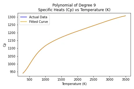
• This part plots the actual data points (T vs cp) in blue and the fitted curve in orange.
• It sets the title, labels for the axes, legend, and displays the plot.
• plot_counter variable is introduced to keep track of plot numbers.
• plt.savefig() is used to save the plot as an image file with a filename based on the polynomial degree.
• plot_counter is incremented to keep track of the plot number.

Plot Residuals and Temperature and Saves Plot as Image Files

    # Plot residuals
    plt.plot(T, residuals, color='red', label='Residuals')
    plt.axhline(y=0, color='gray', linestyle='--')
    plt.title('Polynomial of Degree ' + str(I) + '\nResiduals vs Temperature (K)')
    plt.xlabel('Temperature (K)')
    plt.ylabel('Residuals')
    plt.legend()
    plt.tight_layout()
    
    # Save the plot
    plt.savefig('plot_' + str(I) + '_residuals.png')
    
    # Increment the plot counter
    plot_counter += 1
    
    # Display plot
    plt.show()

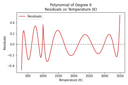
• This part plots the residuals (difference between actual data and fitted curve) against temperature.
• A horizontal dashed line is added at y=0 for reference.
• It sets the title, labels for the axes, legend, and displays the plot.
• plot_counter variable is introduced to keep track of plot numbers.
• plt.savefig() is used to save the plot as an image file with a filename based on the polynomial degree.
• plot_counter is incremented to keep track of the plot number.

Print Fitness Characteristics:

    # Print fitness characteristics
    print("\nPolynomial of Degree {}: ".format(I))
    print("  - SSE: {:.4f}".format(SSE))
    print("  - SSR: {:.4f}".format(SSR))
    print("  - SST: {:.4f}".format(SST))
    print("  - R_squared: {:.4f}".format(R_squared))

• This part prints out the fitness characteristics for the current polynomial degree.
• It displays the degree of the polynomial, SSE, SSR, SST, and R-squared values.

The loop continues for polynomial degrees from 1 to 9, and each time it fits a polynomial of a different degree to the data and evaluates its performance through the fitness characteristics. Finally, it plots the actual data, the fitted curve, and the residuals, providing visual insights into the quality of the fit. The code now generates and saves two plots for each polynomial degree: one showing the actual data and the fitted curve, and the other showing the residuals. The filenames for the saved plots indicate the polynomial degree and the type of plot. The plot counter ensures unique filenames for each plot.

Explanation of the results whether they are good or bad:

Based on the polynomial degree I provided in the code (9), the results are relatively good. The polynomial of degree 9 is able to closely follow the actual data points in the plot. The orange line in the plot represents the fitted curve.

However, it's important to note that fitting a high-degree polynomial to the data may result in overfitting. This means that the polynomial model becomes too complex, including even small random fluctuations in the data. As a result, the fitted curve might deviate too much from the actual data.

In the plot, the blue line represents the actual data points, and the orange line represents the fitted curve. The two curves are close, indicating a good fit.

5. What needs to be done in order to make the curve fit perfect?

To achieve a perfect curve fit, where the fitted curve exactly matches the actual data points, several considerations can be inferred from the provided code:

1. Choose the Right Model Degree: In the code, polynomial functions of degrees 1 to 9 are considered. Choosing the correct degree of polynomial is crucial. If the degree is too low, the model might underfit the data, and if it's too high, it might overfit. One way to potentially improve the fit is to experiment with different polynomial degrees and select the one that best fits the data.
2. Improve the Model Equation: The polynomial function defined in the code is limited to pure polynomial terms. However, real-world data might exhibit non-polynomial behavior. In such cases, considering more complex equations or combining polynomial terms with other functions might improve the fit.
3. Optimize Curve Fitting Parameters: The code uses curve_fit from SciPy to perform the curve fitting. This function attempts to find the optimal parameters for the polynomial function. Fine-tuning the optimization process, such as adjusting the method or tolerance, might lead to a better fit.
4. Data Preprocessing: Preprocessing the data before fitting the curve can help improve the fit. Techniques such as smoothing noisy data, removing outliers, or transforming the data might enhance the accuracy of the curve fit.
5. Regularization: To prevent overfitting, regularization techniques like adding penalties to the parameters or using a Bayesian approach can be applied. This ensures that the fitted curve generalizes well to unseen data.
6. Increase Data Resolution: Adding more data points, especially in regions where the fit is poor, can enhance the accuracy of the curve fit. However, this might not always be feasible or practical depending on the availability of data.
7. Iterative Improvement: After fitting the curve, analyzing the residuals and iterating through the fitting process with adjustments based on the insights gained can lead to a better fit.

By considering these factors and iteratively refining the curve fitting process, one can potentially move towards achieving a closer-to-perfect fit between the fitted curve and the actual data. However, it's important to note that achieving a truly perfect fit might not always be possible due to inherent limitations in the data and modeling assumptions.

6. Show empirically as to how well your curve has been fit.

SSE (Sum of Squares Error):

• SSE measures the total squared difference between the actual observed values and the predicted values by the model.
• It quantifies the discrepancy between the actual data points and the fitted curve.

`SSE = n sum_(i=1)^n( Y(i)- f(x_i))^2`

Where:

• Y(i) is the observed value of the dependent variable at input xi​.
• f(xi​) is the predicted value of the dependent variable at input xi​.
• n is the number of data points.

SSR (Sum of Squares Regression):

• SSR measures the total squared difference between the fitted values and the mean of the observed values.
• It represents the portion of the total variation in the dependent variable that is explained by the regression model.

`SSR = n sum_(i=1)^n (f(x_i) - Mean)^2`

Where:

• f(xi​) is the predicted value of the dependent variable at input xi​.
• Mean is the mean of the observed values of the dependent variable.
• n is the number of data points.

SST (Total Sum of Squares):

• SST measures the total squared difference between the observed values and their mean.
• It represents the total variation in the dependent variable.
• SST can be decomposed into SSR and SSE:

`SST = SSR + SSE`

R-squared (Coefficient of Determination):

• R-squared is a statistical measure that represents the proportion of the variance for a dependent variable that's explained by an independent variable or variables in a regression model.
• It ranges from 0 to 1, where 0 indicates that the model explains none of the variability of the response data around its mean, and 1 indicates that the model explains all the variability of the response data around its mean.

`R^2 = (SSR) / (SST)`

In conclusion, understanding SSE, SSR, SST, and R-squared is crucial in evaluating the performance and effectiveness of a regression model. Together, these metrics offer insights into the goodness-of-fit of a regression model and help assess its predictive power.

Output:

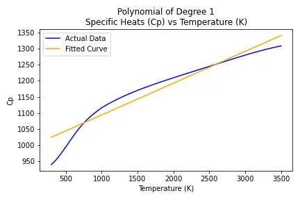
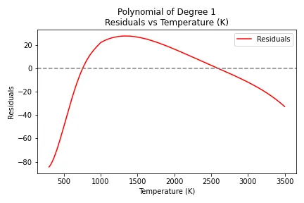
Polynomial of Degree 1:

- SSE: 2163049.0892

- SSR: 26630624.1604

- SST: 28793673.2496

- R_squared: 0.9249

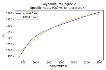
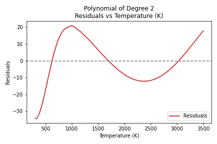
Polynomial of Degree 2:

- SSE: 540107.5629

- SSR: 28253565.6877

- SST: 28793673.2506

- R_squared: 0.9812

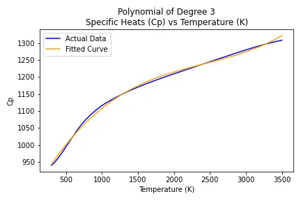
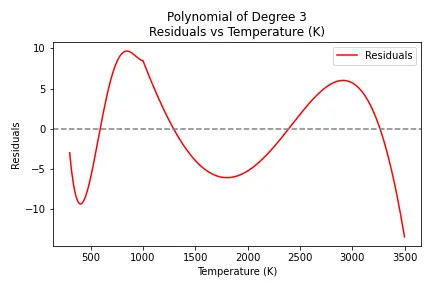
Polynomial of Degree 3:

- SSE: 94272.0205

- SSR: 28699401.2357

- SST: 28793673.2562

- R_squared: 0.9967

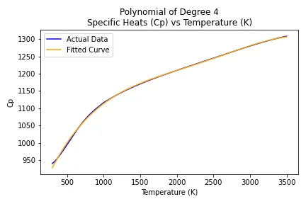
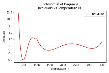
Polynomial of Degree 4:

- SSE: 11070.2748

- SSR: 28782602.9777

- SST: 28793673.2525

- R_squared: 0.9996

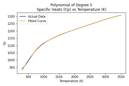
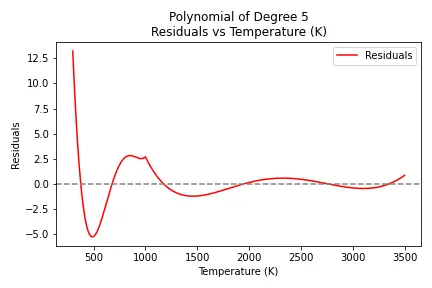
Polynomial of Degree 5:

- SSE: 10807.2677

- SSR: 28782865.9846

- SST: 28793673.2523

- R_squared: 0.9996

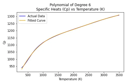
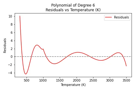
Polynomial of Degree 6:

- SSE: 8332.2327

- SSR: 28785341.0172

- SST: 28793673.2499

- R_squared: 0.9997

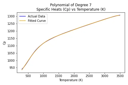
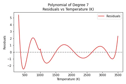
Polynomial of Degree 7:

- SSE: 3691.6255

- SSR: 28789981.6581

- SST: 28793673.2836

- R_squared: 0.9999

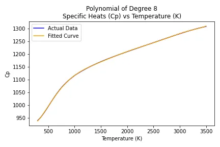
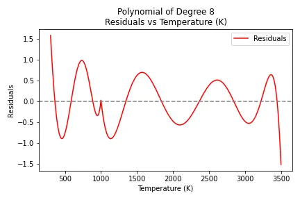
Polynomial of Degree 8:

- SSE: 832.2498

- SSR: 28792840.9887

- SST: 28793673.2385

- R_squared: 1.0000

Polynomial of Degree 9:

- SSE: 95.8326

- SSR: 28793576.9930

- SST: 28793672.8256

- R_squared: 1.0000

Conclusion:

The curve fitting analysis performed on the Specific Heats (Cp) vs Temperature (K) data using polynomials of degrees 1 to 9, it is observed that as the degree of the polynomial increases, the sum of squared errors (SSE) decreases, and the coefficient of determination (R-squared) approaches 1, indicating a better fit. However, a higher degree polynomial may lead to overfitting, and a balance must be struck between the complexity of the model and its accuracy. The residuals, which represent the difference between the actual data and the fitted curve, are generally small and randomly distributed, suggesting that the fitted curves are a good representation of the data. Overall, the polynomial of degree 9 provides the best fit, but a lower degree polynomial may be more appropriate depending on the desired level of complexity and the potential for overfitting.