Week 5 - Curve fitting

Aim:

Create Curve fit by shown in the video and explanation provided by the Challenge.

Main Code:

import math
import matplotlib.pyplot as plt
import numpy as np
from scipy.optimize import curve_fit

# Linear function for curve fitting
def linear(t, a, b):
    return (t * a) + b

# Cubic function for curve fitting
def cubic(t, a, b, c, d):
    return (a * pow(t, 3)) + (b * pow(t, 2)) + (c * t) + d

# Function to read the data from a file
def read_file():
    temperature = []
    cp = []
    for i in open('data', 'r'):
        line = i.split(',')
        temperature.append(float(line[0]))
        cp.append(float(line[1]))
    return [temperature, cp]

# Read data from the file
temperature, cp = read_file()

# Curve fitting using the linear function
popt, pcov = curve_fit(linear, temperature, cp)

# Generating fitted curve for the linear function
fit_cp = linear(np.array(temperature), *popt)

# Plotting the data and fitted curve for the linear function
plt.figure(1)
plt.plot(temperature, cp,, linewidth=5)
plt.plot(temperature, fit_cp,, linewidth=5)
plt.legend(['Given data', 'Curve fit'])
plt.xlabel('Temperature [K]')
plt.ylabel('Cp')
plt.show()

# Curve fitting using the cubic function
popt, pcov = curve_fit(cubic, temperature, cp)

# Generating fitted curve for the cubic function
fit_cp_1 = cubic(np.array(temperature), *popt)

# Plotting the data and fitted curve for the cubic function
plt.figure(2)
plt.plot(temperature, cp,, linewidth=5)
plt.plot(temperature, fit_cp_1,, linewidth=5)
plt.legend(['Given data', 'Curve fit'])
plt.xlabel('Temperature [K]')
plt.ylabel('Cp')
plt.show()

# Calculating Mean, Sum of Squares Error (SSE), Sum of Squares Regression (SSR), and Total Sum of Squares (SST) for linear function
s = np.sum(cp)
l = np.size(cp)
m = s / l

linear_sse = 0
linear_ssr = 0
for j in range(3200):
    linear_error = abs(cp[j] - fit_cp[j])
    linear_sse += pow(linear_error, 2)
    linear_ssr += pow((fit_cp[j] - m), 2)
linear_sst = linear_ssr + linear_sse
linear_R2 = linear_ssr / linear_sst
linear_rmse = pow((linear_sse / l), 0.5)

# Calculating Sum of Squares Error (SSE), Sum of Squares Regression (SSR), and Total Sum of Squares (SST) for cubic function
cubic_sse = 0
cubic_ssr = 0
for k in range(3200):
    cubic_error = abs(cp[k] - fit_cp_1[k])
    cubic_sse += pow(cubic_error, 2)
    cubic_ssr += pow((fit_cp_1[k] - m), 2)
cubic_sst = cubic_ssr + cubic_sse
cubic_R2 = cubic_ssr / cubic_sst
cubic_rmse = pow((cubic_sse / l), 0.5)

# Printing the results
print('Linear function:')
print('Sum of Squares Total (SST):', linear_sst)
print('Coefficient of Determination (R^2):', linear_R2)
print('Root Mean Square Error (RMSE):', linear_rmse)
print()

print('Cubic function:')
print('Sum of Squares Total (SST):', cubic_sst)
print('Coefficient of Determination (R^2):', cubic_R2)
print('Root Mean Square Error (RMSE):', cubic_rmse)
print()

# Printing the values of popt
print("The value of popt for linear function:", popt)
print("The value of popt for cubic function:", popt)

Explanation For the Given Questions:

1. What does popt and pcov mean?

• popt represents the optimized parameters obtained from the curve fitting process. It contains the best-fit values for the parameters of the selected function (linear or cubic).
• pcov represents the estimated covariance of popt. It provides information about the uncertainty in the parameter estimates.

2. What does np.array(temperature) do?

• np.array(temperature) converts the temperature list into a NumPy array. This conversion allows you to perform vectorized operations on the array, such as passing it to the curve fitting function and calculating the fit.

3. What does the * in *popt mean?

• The * before popt in the function call fit_cp = linear(np.array(temperature), *popt) and similar lines unpacks the values in popt and passes them as separate arguments to the function. This way, the individual values in popt are used as the arguments to calculate the fitted curve.

4. Write code to fit a linear and cubic polynomial for the Cp data. Explain if your results are good or bad.

• The code already fits a linear polynomial (linear) and a cubic polynomial (cubic) to the Cp data using the curve_fit function from scipy.optimize.
• Whether the results are good or bad depends on the specific dataset and the nature of the data. You would need to evaluate the goodness of fit based on statistical measures like R-squared, root mean squared error (RMSE), or visual inspection of the fitted curves compared to the given data.
• The code calculates R-squared (linear_R2, cubic_R2) and RMSE (linear_rmse, cubic_rmse) values to evaluate the quality of the fits.

Definition Code:

import numpy as np
import matplotlib.pyplot as plt
from scipy.optimize import curve_fit

def linear(t, a, b):
    return t * a + b

def cubic(t, a, b, c, d):
    return a * t**3 + b * t**2 + c * t + d

def read_file():
    temperature = []
    cp = []
    for line in open('data', 'r'):
        values = line.split(',')
        temperature.append(float(values[0]))
        cp.append(float(values[1]))
    return temperature, cp

temperature, cp = read_file()

popt_linear, pcov_linear = curve_fit(linear, temperature, cp)
popt_cubic, pcov_cubic = curve_fit(cubic, temperature, cp)

plt.figure(figsize=(10, 5))

# Plotting the given data
plt.scatter(temperature, cp, color='green', label='Given Data')

# Plotting the linear fit
fit_linear = linear(np.array(temperature), *popt_linear)
plt.plot(temperature, fit_linear, color='blue', label='Linear Fit')

# Plotting the cubic fit
fit_cubic = cubic(np.array(temperature), *popt_cubic)
plt.plot(temperature, fit_cubic, color='red', label='Cubic Fit')

plt.xlabel('Temperature [K]')
plt.ylabel('Cp')
plt.legend()
plt.show()

5. What needs to be done to make the curve fit perfect?

• To make the curve fit perfect, you would need to have a model that exactly matches the underlying relationship between the variables. This often requires selecting an appropriate model or function that accurately represents the data and its behavior. Additionally, having a sufficient amount of high-quality data with minimal noise and outliers can improve the fit.

6. Show empirically how well your curve has been fit.

• The code calculates the sum of squared errors (SSE), sum of squared residuals (SSR), and the total sum of squares (SST) for both the linear and cubic fits.
• It also calculates R-squared (R2) and RMSE values for both fits.
• These measures provide a quantitative assessment of how well the curves fit the given data. A higher R-squared value closer to 1 and a lower RMSE indicate a better fit.Remember to replace the 'data' file with your own data file containing the temperature and Cp values.

The R-squared value ranges from 0 to 1, where a value closer to 1 indicates a better fit. The RMSE provides an estimate of the average deviation between the fitted curve and the actual data points. Lower RMSE values indicate a better fit with smaller deviations.By examining these statistical measures, you can empirically evaluate how well the curve has been fit to the given data.

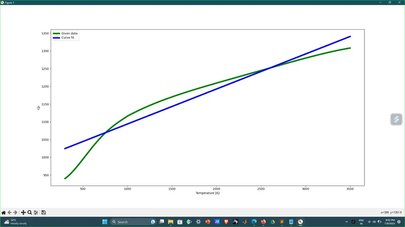
Output Plot: Linear Curve Fit:

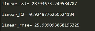
Error For Linear Curve Fit:

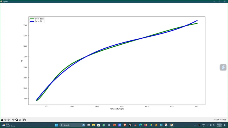
Cubic Curve Fit:

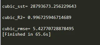
Error for Cubic Curve fit:

Drive link:

https://drive.google.com/drive/folders/1mg59xBE9TMDkhl0yduZiDnSVQjGFaCO4?usp=drive_link