Week 5 - Curve fitting

AIM:
Write a Python code for Curve fitting.

THEORY:
Curve fitting is the process of constructing a curve, or mathematical function, that has the best fit to a series of data points, possibly subject to constraints. Curve fitting can involve either interpolation, where an exact fit to the data is required, or smoothing, in which a "smooth" function is constructed that approximately fits the data. It examines the relationship between one or more predictors (independent variables) and a response variable (dependent variable), with the goal of defining a "best fit" model of the relationship.

How to choose the best fit?

Upon finding a curve that satisfies the data points there are 4 quantities that help us measure the goodness of fit criteria or how well the equation is representing the data points. They are listed as: -

• The sum of squares due to error (SSE)
• R-Square
• Adjusted R-Square
• Root Mean Square error (RMSE)

How to make a curve fit perfectly?

In order to have a curve fit perfectly over the data points provided, the error should be negligible, i.e. the values of R-Square should be exactly ‘1’. Generally, the minimal error is taken into account for the best fit but to obtain a perfect fit, all the errors including centering and scaling errors should be nulled.

How to get the best fit?

A line of best fit can be roughly determined using an eyeball method by drawing a straight line on a scatter plot so that the number of points above the line and below the line is about equal (and the line passes through as many points as possible).

Also, the Split Polynomial technique can opt to obtain a curve fit closest to the data set. This is one of the most viable techniques to be performed for best fit.

What could be done to improve the cubic fit?

• Increase the number of iterations or function evaluations allowed.
• Reduce the convergence tolerance.
• Try also sub-setting the data and fitting different subsets of data separately.

OBJECTIVE:

1. What does popt and pcov mean? (Watch the video to get some context)

* 'popt'-
Generally refers to an array of optimal readings or values for the given declared parameters which helps to minimize the sum of the squares of the leftover values.

* 'pcov'-
A two-dimensionally array that contains the estimated covariance of popt. The diagonals provide the variance of the parameter estimate.

2. What does np.array(temperature) do?

" np.array(temperature) " - The function that stores the values of the temperature as an array and then passes it to the numpy function.

3. What does the * in *popt mean?

• popt contains values of a,b,c..etc.
• *popt helps to refer to the values in popt.
• '*" in ' *popt ' is used to call the arguments i.e irrespective of calling each coefficient individually, *popt is used to call all the coefficients in a single call in a function

4. Write code to fit a linear and cubic polynomial for the Cp data. Explain if your results are good or bad.

Linear polynomial equation:

import numpy as np 
import matplotlib.pyplot as plt 
from scipy.optimize import curve_fit


# Curve fit function
def func(t,a,b,c):  # a,b,c are constants
	return a*t + b*t + c    # Linear polynomial equation

# Reading thermodynamic data file 
def read_file():
		temperature = []
		cp = []
		for line in open ('data.txt','r'):  # data.txt is a file stored with the temperature and specific heat.
				values = line.split(',')
				temperature.append(float(values[0]))  
				cp.append(float(values[1]))
		return [ temperature, cp ]
# Main Program
temperature, cp = read_file()
popt, pcov = curve_fit(func, temperature,cp)		
fit_cp = func(np.array(temperature), *popt)

plt.plot(temperature,cp, linewidth=2)
plt.plot(temperature, fit_cp,linewidth=2)
plt.legend(['Actual Data', 'Curve fit'])
plt.xlabel('Temperature')
plt.ylabel('Cp')
plt.grid()
plt.show()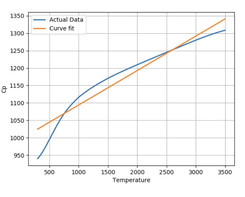

Cubic polynomial equation:

import numpy as np 
import matplotlib.pyplot as plt 
from scipy.optimize import curve_fit


# Curve fit function
def func(t,a,b,c,d):  #a,b,c are constants

	return a*pow(t,3) + b*pow(t,2) + c*t + d    # CUBIC EQUATION- ax^3+bx^2+cx+d=0   here x=t

# Reading thermodynamic data file 
def read_file():
		temperature = []
		cp = []
		for line in open ('data.txt','r'):
				values = line.split(',')
				temperature.append(float(values[0]))
				cp.append(float(values[1]))
		return [ temperature, cp ]
# Program
temperature, cp = read_file()
popt, pcov = curve_fit(func, temperature,cp)		
fit_cp = func(np.array(temperature), *popt)

plt.plot(temperature,cp,linewidth=2)
plt.plot(temperature, fit_cp,linewidth=2)
plt.legend(['Actual Data', 'Curve fit'])
plt.xlabel('Temperature')
plt.ylabel('Cp')
plt.grid()
plt.show()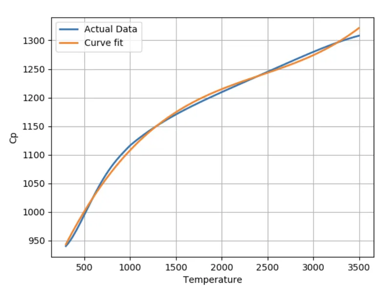

From both cases, it is observed that the linear polynomial equation of the graph obtained for temperature vs Cp showed that there is more difference in trend between the actual data and the curve fit.

Whereas for the cubic polynomial equation, the graph obtained for temperature vs Cp showed that there is a close curve-fit trend when compared to linear polynomial curve-fit trends.

5. What needs to be done in order to make the curve fit perfectly?

• By increasing the degree of the curve we can make the best curve fit.
• If we further increase the degree of the curve to 4 then the curve will be more accurate than the cubic polynomial.
• Further increasing the degree of the polynomial will increase the calculating complexity and time required, hence 4th order polynomial can be taken as a sufficient curve fit.