Week 2.1 Solving Air standard cycle using MATLAB.

AIM:

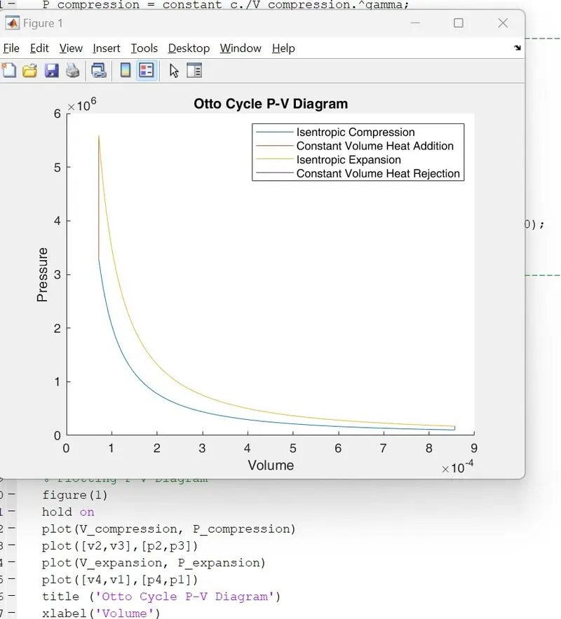
Write code that can solve an otto cycle and make plots for it.

Challenge expectation:

• Code should create a PV diagram,
• Code output should display the thermal efficiency of the engine.

CONCEPT:

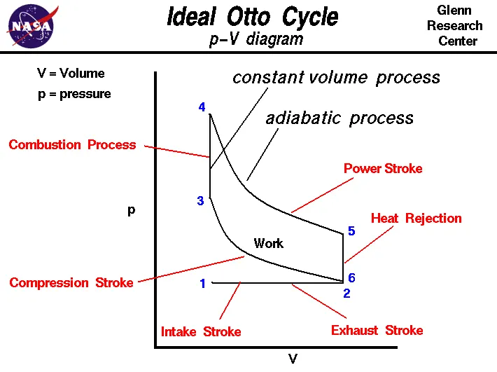
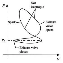
IDEAL ACTUAL

THEORY :

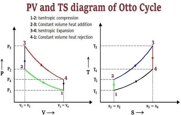
The starting point is the general expression for the thermal efficiency of a cycle:

The convention, as previously, is that heat exchange is positive if heat is flowing into the system or engine, so is negative. The heat absorbed occurs during combustion when the spark occurs, roughly at constant volume. The heat absorbed can be related to the temperature change from state 2 to state 3 as:

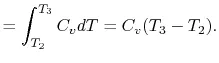The heat rejected is given by (for a perfect gas with constant specific heats)

Substituting the expressions for the heat absorbed and rejected in the expression for thermal efficiency yields

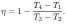
We can simplify the above expression using the fact that the processes from 1 to 2 and from 3 to 4 are isentropic:

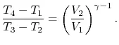
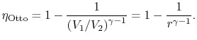
The quantity is called the compression ratio. In terms of compression ratio, the efficiency of an ideal Otto cycle is:

FUNCTION CODE:

function [V] = engine_kinematics(bore, stroke, con_rod, cr, start_crank, end_crank)

% Crank Pin Radius-
a = stroke/2;
% Ratio of Connecting Rod and Crank Pin Radius-
R = con_rod/a;

% Swept Volume Calculations-
v_s = (pi/4)*bore^2*stroke;
% Clearance Volume Calculations-
v_c = v_s/(cr-1);

theta = linspace(start_crank,end_crank,100);

% Combustion Voulme Formula Calculations- 
term1 = 0.5*(cr-1);
term2 = R +1 - cosd(theta);
term3 = (R^2 - sind(theta).^2).^0.5;

V = (1 + term1*(term2 - term3)).*v_c;

end

• Here we have created a Function filed name engine_kinematics which assigns value to the output array.
• For inputs added different Inputs like the Crankpin radius, Ratio of connecting rod, and crankpin radius.
• Using the formula of Swept Volume and Clearance Volume calculated the value respectively.
• Using linspace command created an array for different values of theta.
• For Calculation of Combustion Volume (V) divided the formula into three parts term1, term2, and term3, and finally combined into a main single formula. (V)
• linspace - The linspace function generates linearly spaced vectors.
  
  

Code for Thermal Efficiency and PV Diagram :

clear all
close all
clc

% INPUTS-
gamma = 1.4;
t3 = 2300;

% State variables at state point 1-------------------------------
p1 = 101325;
t1 = 500;

% Engine geometric parameters-
bore = 0.1;
stroke = 0.1;
con_rod = 0.15;
cr = 12;

% Calculating the swept volume and the clearance volume-
v_swept = (pi/4)*bore^2*stroke;
v_clearance = v_swept/(cr-1);

%Volume at Stage 1 and 2-
v1 = v_swept + v_clearance;
v2 = v_clearance;

% State variables at state point 2----------------------------------

% p2v2^gamma = p1v1^gamma | p2 = p1*(v1/v2)^gamma = p1*cr^gamma
p2 = p1*cr^gamma;

% Temperature at point 2-
%p1v1/t1 = p2v2/t2 | t2 = p2*v2*t1/(p1*v1)
t2 = p2*v2*t1/(p1*v1);

% For Constant (C)-
constant_c = p1*v1^gamma;

% For compression Stroke Volume and Pressure Calculation-
V_compression = engine_kinematics(bore, stroke, con_rod, cr, 180, 0);
P_compression = constant_c./V_compression.^gamma;

% State variables at point 3-------------------------------------------
v3 = v2;

%Pressure at point 3-
%p3v3/t3 = p2v2/t2 | p3 = p2*t3/t2
 p3 = p2*t3/t2;

% For Constant (C)-
constant_c = p3*v3^gamma;

% For compression Stroke Volume and Pressure Calculation-
V_expansion = engine_kinematics(bore, stroke, con_rod, cr, 0, 180);
P_expansion = constant_c./V_expansion.^gamma;

% State vairiables at state point 4-------------------------------------
v4 = v1;

% Pressure at point 4-
%p3v3^gamma = p4v4^gamma | p4 = p3(v3/v4)^gamma
 p4 = p3*(v3/v4)^gamma;
 

 % Formula for Thermal Efficiency
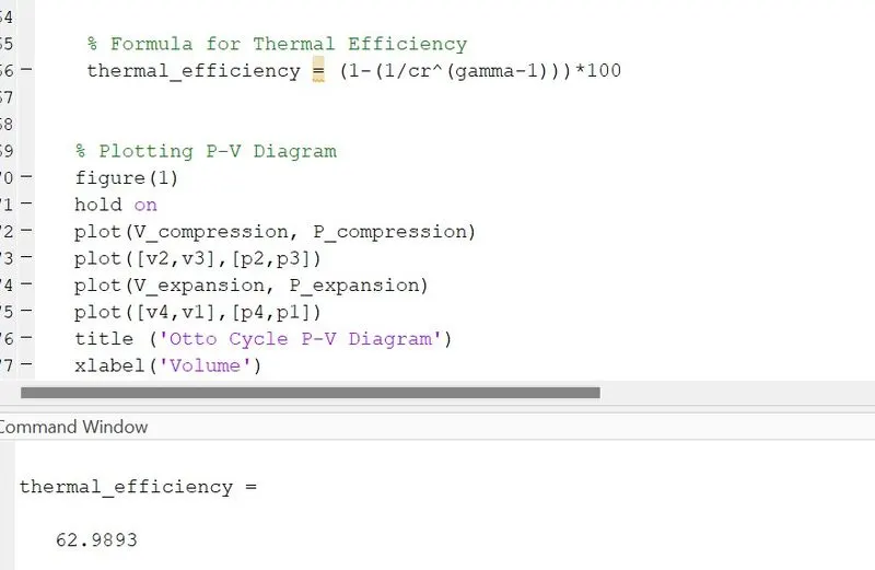
 thermal_efficiency = (1-(1/cr^(gamma-1)))*100 
 
 
% Plotting P-V Diagram
figure(1)
hold on
plot(V_compression, P_compression)
plot([v2,v3],[p2,p3])
plot(V_expansion, P_expansion)
plot([v4,v1],[p4,p1])
title ('Otto Cycle P-V Diagram')
xlabel('Volume')
ylabel('Pressure')
legend ('Isentropic Compression','Constant Volume Heat Addition','Isentropic Expansion','Constant Volume Heat Rejection')

• clear all - To clear all the variables from the current workspace.
• clc - clear all the texts from the command window.
• close all - Close all figures whose handles are visible.
• plot - This command is used to Plot Graph.
• linewidth - The line width command is given to the width of the line which is going to be plotted on a graph.
• title - For giving title to the graph.
• legend - It is used for indication of the line.
• axis - For assigning axis to the plot.
• hold on - Command stops MATLAB execution temporarily.
• INPUTS VALUES: gamma, t3, p1, and t1.
• After giving inputs we added the geometric parameters. (bore, stroke, connecting rod, and compression ratio)
• Wrote formulae for swept volume and clearance volume, and calculated v1 and v2. (For stages 1 and 2)
• Now, for stage 2 wrote formula for p2 and t2 and calculated t2 and p2.
• Using the 'constant_c' we can easily calculate the compression stroke volume and Compression stroke pressure.
• At stage three calculate the value for 'v3'.
• Again using 'constant_c' and calculating the 'Expansion stroke volume' and 'Expansion stroke pressure'.
• For the final stage, using the formula calculating the values for 'v4' and 'p4'.
• Now calculate the thermal Efficiency using the formula.
  (1-(1/cr^(gamma-1)))*100 )
• Finally, Plotting the P-V Diagram for (v_compression,V_expansion,v1,v2,v3,v4) and (p_compression,p_expansion,p1,p2,p3,p4).
• Used basic commands for labeling like xlabel, ylabel, title, and legend.

RESULTS:

ERRORS WHILE PROGRAMMING:

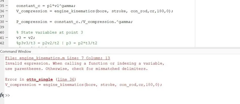
• Errors faced while coding -

1.) Typing mistake in Thermal Efficiency spellings.

2.) Line 36: In V_compression the spelling of con_rod was typed cond_rod and In function, the code forgot to add the multiplication symbol(*).

(v_s = (pi/4)bore^2*stroke), correct formula: (v_s = (pi/4)*bore^2*stroke)