Week 4.1 - Genetic Algorithm using MATLAB
Aim:
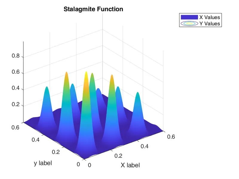
Write the code in MATLAB to optimize the stalagmite function and find out the global maxima of the function.
Challenge expectation:
- Clearly explain the concept of genetic algorithm in your own words and also explain the syntax for ga in MATLAB in your report.
- Make sure that your code gives the same output, even if it is made to run several times.
- Plot graphs for all three studies and for F maximum vs no. of iterations.
CONCEPT:
A genetic algorithm (GA) is a search-based optimization technique based on the principles of Genetics and Natural Selection. It is frequently used to find optimal or near-optimal solutions to difficult problems which otherwise would take a lifetime to solve. It is frequently used to solve optimization problems, in research, and in machine learning.
A genetic algorithm (GA) is a search-based optimization technique based on the principles of Genetics and Natural Selection. It is frequently used to find optimal or near-optimal solutions to difficult problems which otherwise would take a lifetime to solve. It is frequently used to solve optimization problems, in research, and in machine learning.
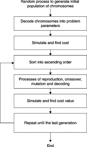
It basically involves five phases to solve the complex optimization problems, which are given below:
- Initialization
- Fitness Assignment
- Selection
- Reproduction
- Termination
Advantages of GAs
GAs have various advantages which have made them immensely popular. These include −
-
Does not require any derivative information (which may not be available for many real-world problems).
-
Is faster and more efficient compared to the traditional methods.
-
Has very good parallel capabilities.
-
Optimizes both continuous and discrete functions and also multi-objective problems.
-
Provides a list of “good” solutions and not just a single solution.
-
Always gets an answer to the problem, which gets better over time.
-
Useful when the search space is very large and there are a large number of parameters involved.
Limitations of GAs
Like any technique, GAs also suffer from a few limitations. These include −
-
GAs are not suited for all problems, especially problems that are simple and for which derivative information is available.
-
The fitness value is calculated repeatedly which might be computationally expensive for some problems.
-
Being stochastic, there are no guarantees of the optimality or the quality of the solution.
-
If not implemented properly, the GA may not converge to the optimal solution.
SYNTAX FOR GA:
x = ga(fun,nvars)x, to the objective function, fun. nvars is the dimension (number of design variables) of fun.x = ga(fun,nvars,A,b,Aeq,beq)x to fun, subject to the linear equalities Aeq*x = beq and A*x ≤ b. (Set A=[] and b=[] if no linear inequalities exist.) ga evaluates the matrix product Aeq*x as if x is transposed (Aeq*x').
x = ga(fun,nvars,A,b,Aeq,beq,lb,ub)x, so that a solution is found in the range lb ≤ x ≤ ub. (Set Aeq=[] and beq=[] if no linear equalities exist.)
x = ga(fun,nvars,A,b,Aeq,beq,lb,ub,nonlcon)nonlcon. The function nonlcon accepts x and returns vectors C and Ceq, representing the nonlinear inequalities and equalities respectively. ga minimizes the fun such that C(x) ≤ 0 and Ceq(x) = 0. (Set lb=[] and ub=[] if no bounds exist.)
OUTPUT OF SYNTAX:
[, for any previous input arguments, also returns x,fval] = ga(___)fval, the value of the fitness function at x.
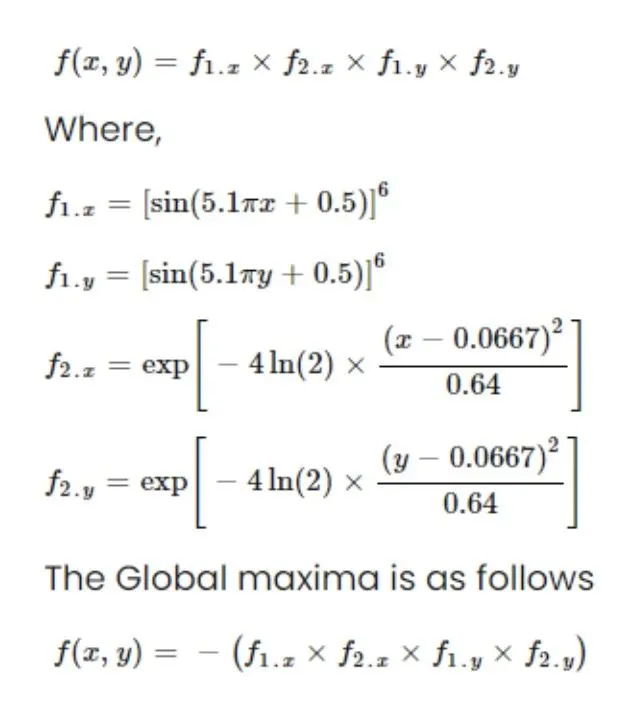
PROCEDURE:
- Function code :
% Stalagmite Function

function [f] = stalagmite_challenge(inputs)

x = inputs(1);
y = inputs(2);

% Converting Genetic Alogorithm into Matlab Formula.

f1 = (sin(5.1*pi*x + 0.5)).^6;
f2 = exp(-4*log(2)*((x-0.0667).^2)./0.64);
f3 = (sin(5.1*pi*y + 0.5)).^6;
f4 = exp(-4*log(2)*((y-0.0667).^2)./0.64);

% Global Maxima Formula

f = -(f1*f2*f3*f4);

end- Main code :
clear all
close all
clc

%INPUTS
lower_bound = input('Enter the Lower Bound Value: ');
upper_bound = input('Enter the Upper Bound Value: ');

% Input Variables with linespace
x = linspace(lower_bound,upper_bound,150);
y = linspace(lower_bound,upper_bound,150);

% 3D MESH Creation
[xx, yy] = meshgrid(x,y);

% Giving the Count
count = 50;

tic                      % Tic starts the clock time for the function
for i = 1:length(xx)     % Now starting the For Loop
    for j = 1:length(yy)
        input_vector(1)= xx(i,j);
        input_vector(2)= yy(i,j);
        f(i,j)=stalagmite(input_vector);
    end
end

% TOC stops the timer and shows the end time
study_time = toc;

figure(1)
surfc(xx,yy,-f)
shading interp
xlabel('X label')
ylabel('y label')
legend('X Values','Y Values')
title('Stalagmite Function')
saveas(1, 'Stalagmite.png')
% [x,fval] = ga(@stalagmite,2)

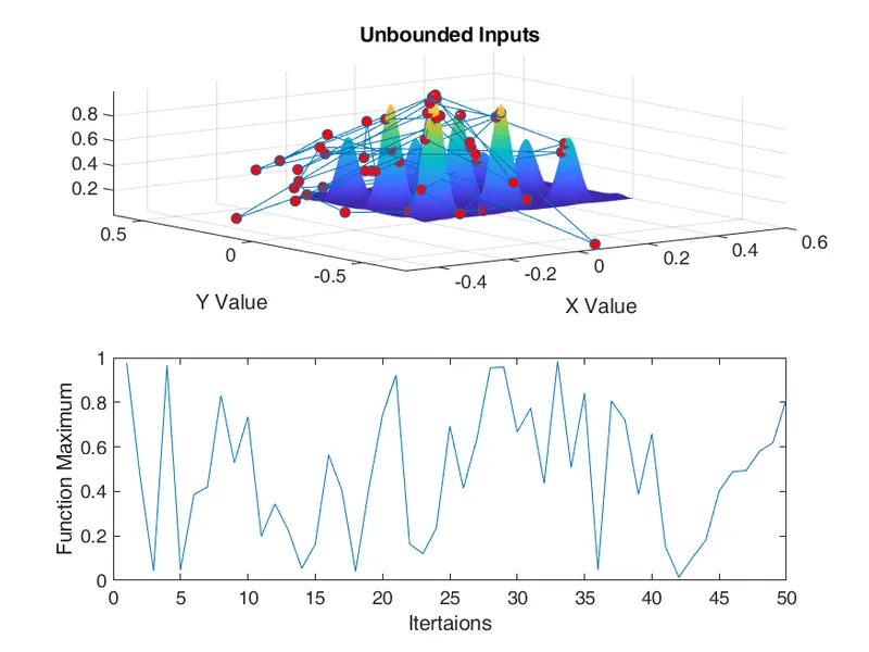
% STUDY 1 -
% UNBOUNDED/RANDOM SAMPLING INPUTS

tic                    % Tic starts the clock time for the function
for i = 1:count        % Now starting the For Loop
    [inputs,fopt(i)] = ga(@stalagmite,2);
    xopt(i) = inputs(1);
    yopt(i) = inputs(2);
end
studytime_1 = toc;

figure(2)
subplot(2,1,1)
surfc(x,y,-f)
shading interp
title('Unbounded Inputs')
xlabel('X Value')
ylabel('Y Value')

hold on

plot3(xopt,yopt,-fopt,'marker','o','markersize',5,'markerfacecolor','r');
subplot(2,1,2)
plot(-fopt)
xlabel('Itertaions')
ylabel('Function Maximum')
saveas(2,'Unbound Inputs.png')

% STUDY 2 -
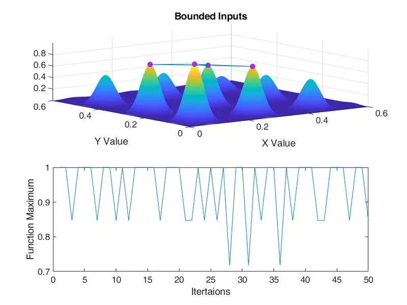
% STATISTICAL BEHAVIOUR WITH UPPER AND LOWER BOUND SAMPLING

tic                     % Tic starts the clock time for the function
for i = 1:count         % Now starting the For Loop
    [inputs,fopt(i)] = ga(@stalagmite,2, [],[],[],[], [lower_bound;lower_bound],[upper_bound;upper_bound]);
    xopt(i) = inputs(1);
    yopt(i) = inputs(2);
end
studytime_2 = toc;

figure(3)
subplot(2,1,1)
surfc(x,y,-f)
shading interp
title('Bounded Inputs')
xlabel('X Value')
ylabel('Y Value')

hold on

plot3(xopt,yopt,-fopt,'marker','o','markersize',5,'markerfacecolor','m');
subplot(2,1,2)
plot(-fopt)
xlabel('Itertaions')
ylabel('Function Maximum')
saveas(3,'Bounded Inputs.png')

% STUDY 3 -
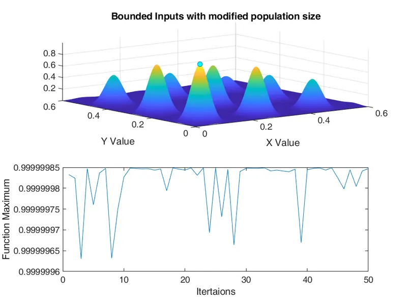
% CODE FOR UPPER AND LOWER BOUND SAMPLING AND INCREASE THE POPULATION
options = optimoptions(@ga);
options = optimoptions(options,'populationsize',170);

tic                     % Tic starts the clock time for the function
for i = 1:count         % Now starting the For Loop
    [inputs,fopt(i)] = ga(@stalagmite,2, [],[],[],[], [lower_bound;lower_bound],[upper_bound;upper_bound],[],[],options);
    xopt(i) = inputs(1);
    yopt(i) = inputs(2);
end
studytime_3 = toc;

figure(4)
subplot(2,1,1)
surfc(x,y,-f)
shading interp
title('Bounded Inputs with modified population size')
xlabel('X Value')
ylabel('Y Value')

hold on

plot3(xopt,yopt,-fopt,'marker','o','markersize',5,'markerfacecolor','c');
subplot(2,1,2)
plot(-fopt)
xlabel('Itertaions')
ylabel('Function Maximum')
saveas(4,'Bounded Inputs with modified population size.png')

% For Finding the Global Maxima
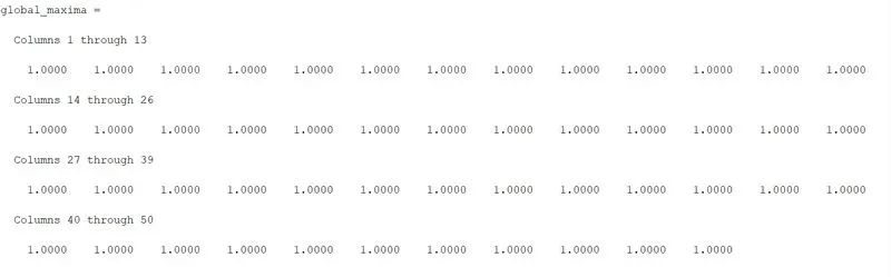
global_maxima = -fopt;
CODE EXPLANATION:
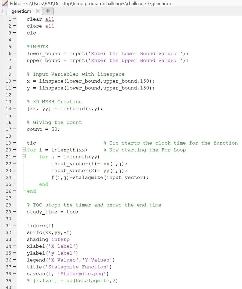
- Giving comments and adding basic commands.
- clear all - To clear all the variables from the current workspace.
- clc - Clear all the texts from the command window.
- close all - Close all figures whose handles are visible.
- The Initial Inputs are given like the lower_bounds and upper_bound. (Using Linspace Commands for X and Y Values)
- linspace - The linspace function generates linearly spaced vectors.
- Now converting into 3D Matrix creation. (Using mesh grid command)
- Using the count command to give the count for no of Iterations.
- A tic command is used to start the clock time for function.
- Now started with the For Loop command and gave the value of the variable "i" and "j".
- Toc command is used to stop the timmer.
- For plotting the basic command are used.
- title - For giving title to the graph.
- legend - It is used for indication of the line.
- axis - For assigning axis to the plot.
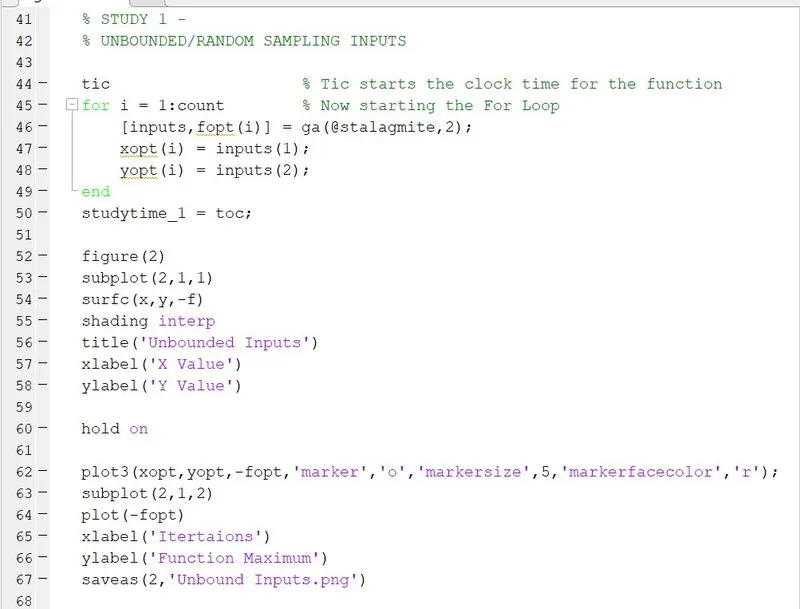
- For UNBOUNDED STALAGMITE,
- ga command is added which finds the minimum of the function.
- For plotting the basic commands are used as subplot, surfc, shading, title, xlabel, ylabel.
- linspace - The linspace function generates linearly spaced vectors.
- plot - This command is used to Plot Graph.
- title - For giving title to the graph.
- legend - It is used for indication of the line.
- axis - For assigning axis to the plot.
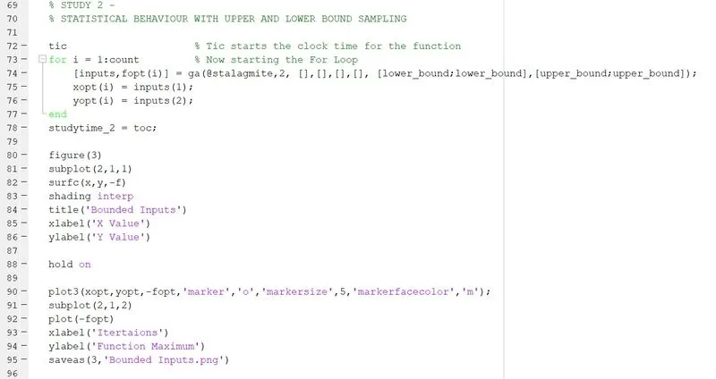
- This is for Study 2 - STATISTICAL BEHAVIOUR WITH UPPER AND LOWER BOUND SAMPLING
- title - For giving title to the graph.
- legend - It is used for indication of the line.
- axis - For assigning axis to the plot.
- Shading - This controls the shading and the color graphic of the objects. (Plot/Graph)
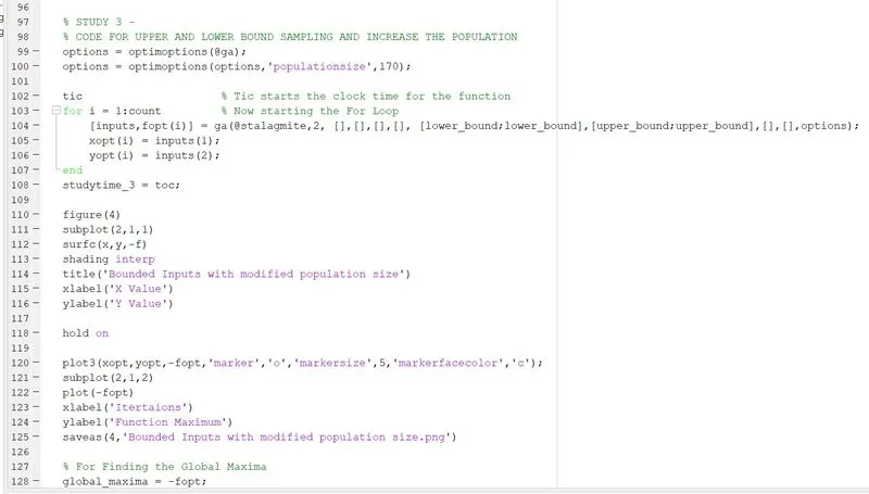
- Study 3 - UPPER AND LOWER BOUND SAMPLING AND INCREASE IN POPULATION
- optimoptions - this command is used to show some options that dont appear sometimes.
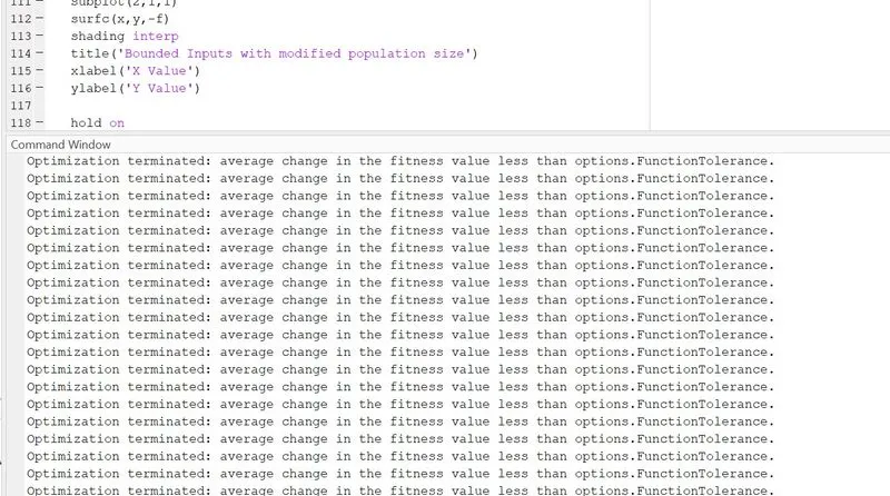
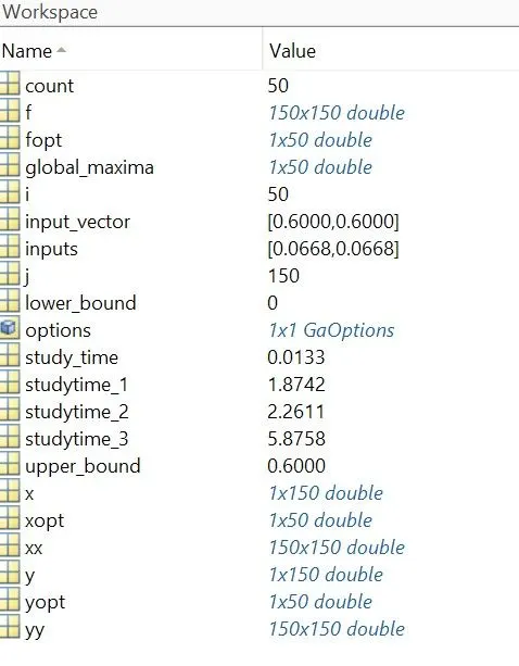
RESULTS:
ERRORS WHILE PROGRAMMING:
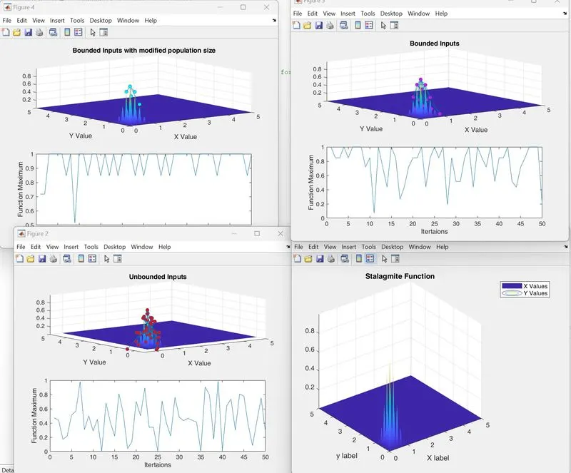
- Entered the Wrong Input values (0 and 5) instead of 0 and 0.6.
CONCLUSIONS:
The above results show that the bounded samples with population size have an accurate solution. This is because the code shows the random samples which can start and end at random points.
To overcome the issues, the bounded samples method is used giving the lower and upper limits. (Therefore, it will take the values which are greater than the upper bound or less than the lower bound.)
This loop gives an output with different Local Maxima with bounded inputs. To conquer this problem, we need to increase the population size as it increases the probability to converge to a global maximum
REFERENCES: