Week 5 - Curve fitting

AIM : To perform curve fitting for linear and cubic polynomial ?

Theory:

Curve fitting: It is the process of formulating a mathematical function that has the best fit for the series of given data points.

Best fit means to construct a curve where the distances between the actual and the predicted values are minimum.

A perfect fit means that the error between the actual and predicted values are zero.

Assume function f(x) to satisfy the data points (x1,y1), (x2,y2).. and so on.

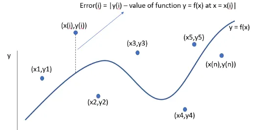
Sum of squared error = `sum_(i=1)^N(y(i)-f(x(i))^2`

If the proposed equation is an nth degree polynomial

`f(x) = A1+ A2*x+A3*x^2+..+underset(" "n)(A)*x^(n-1))`

Differentiating the SSE with each coefficient and equating it to zero will return us the value of the coefficient for which the error is minimum.

Solving the multiple systems of equations we can get the value of the coefficients.

This is the least square error method.

R-square:

`"R square" = (SSR)/(SST)`, where

`SST = SSE + SSR`

SSR stands for the sum of the square of the regression and is equal to the square of the difference between the value of the fitting function at the given point and the mean of the data set.

SSR = `sum_(i=1)^N(f(x(i)-M)^2`, where M is the arithmetic mean of the given data set.

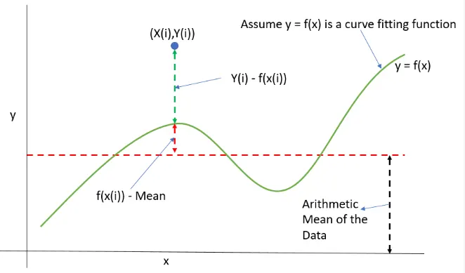
The fit is said to be best if R squared is 1 and worst if 0.

Root Mean squared Error (RMSE):

It is the square root of `"SSE"/n`, where n is the total number of points.

RMSE = `sqrt((sum_(i=1)^N(y(i)-f(x(i)))^2)/n`

1.What is popt and pcov?
popt is an array that stores the values of the coefficient that are being passed in a given function. It gives an array with the optimal values for the parameters so that the sum of the squared residuals of the data is minimized.
pcov is a two-dimensional array that stores the values of the estimated covariance of popt, i.e., the coefficients. It can be used to calculate the standard deviation errors of popt, and is mostly useful when the data has uncertainties.

2.What does np.array(temperature) do in the program?
np.array(temperature) is used for accessing the individual elements of the temperature array with the help of numpy module. This command converts each value of temperature in the data file into an array using the numpy module. The numpy module is imported as np and used to perform mathematical operations like addition, subtraction, multiplication, division, etc. on each element of an array or between the arrays.

3.What does the * in *popt mean?
The * in *popt unpacks the popt array so that the optimized coefficients values can be accessed from the array popt. That is, * aids in referring to all the values stored in the array popt.

4. Write code to fit a linear and cubic polynomial for the Cp data. Explain if your results are good or bad.

Procedure:

• The libraries needed to solve the given problem were imported.
• The equation used to fit the given data set was defined.
• A function to read the file and extract temperature and cp values was made.
• Using the curve_fit function, the optimal values for the coefficients of the fitting equation were determined.
• The cp values were determined by substituting the optimum coefficients and temperature values in the fitting equation.
• Plot was generated to compare the actual curve vs the fit curve and the R squared error for each fit was calculated.
• The best fit was determined among the different functions used based on their R squared value.

#CURVE FITTING FOR LINEAR AND CUBIC POLYNOMIAL

import numpy as np 
import math
import matplotlib.pyplot as plt
from scipy.optimize import curve_fit

# curve fit function(linear)
def func(t,a,b):
	return a*t+b

# curve fit function(cubic polynomial)
def func_3(t,a,b,c,d):
	return a*pow(t,3)+b*pow(t,2)+c*t+d



# Reading the thermodynamic data

def read_file():
	temperature = []
	cp = []
	for line in open('data','r'):
		values = line.split(',')
		temperature.append(float(values[0]))
		cp.append(float(values[1]))
	
	return[temperature,cp]


# main program for  linear polynomial
temperature,cp = read_file()
popt,pcov = curve_fit(func,temperature,cp)
fit_cp = func(np.array(temperature),*popt)

# program for cubic polynomial
temperature,cp = read_file()
popt2,pcov2 = curve_fit(func_3,temperature,cp)
fit_cp2 = func_3(np.array(temperature),*popt2)


#print(popt)
#print(pcov)

# plotting linear polynomial curve fit

plt.plot(temperature,cp,color='green',linewidth=2.5)
plt.plot(temperature,fit_cp,color='blue',linewidth=2.5)
plt.legend(['Actual data','Linear curve fit'])
plt.xlabel('temperature[k]')
plt.ylabel('specific heat at constant pressure Cp')
plt.title('Linear Polynomial Curve Fit')
plt.savefig('plot 1')
plt.grid()
plt.show()

# plotting cubic polynomial curve fit
plt.plot(temperature,cp,color='green',linewidth=2.5)
plt.plot(temperature,fit_cp2,color='blue',linewidth=2.5)
plt.legend(['Actual data','Cubic curve fit'])
plt.xlabel('temperature[k]')
plt.ylabel('specific heat at constant pressure Cp')
plt.title('Cubic Polynomial Curve Fit')
plt.savefig('plot 2')
plt.grid()
plt.show()

# calculation of R-square parameter
SSE = np.sum(pow(np.array((np.array(cp)-np.array(fit_cp))),2))
SSR = np.sum(pow((np.array(np.array(fit_cp)-np.mean(cp))),2))
SST = SSE+SSR;
R_square = SSR/SST;
print('R square for a  splitwise fit 1 = ',R_square)



SSE1 = np.sum(pow(np.array((np.array(cp)-np.array(fit_cp2))),2))
SSR1 = np.sum(pow((np.array(np.array(fit_cp2)-np.mean(cp))),2))
SST1 = SSE1+SSR1;
R_square1 = SSR1/SST1;
print('R square for a  splitwise fit 2 = ',R_square1);

RESULT :

Plot 1:

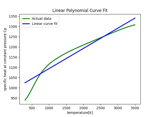
• Represents the Linear curve fit along with raw data.
• The error curve below represents the deviation of specific heat value formed by the linear curve fit from the original value at each value of temperature.

Plot 2:

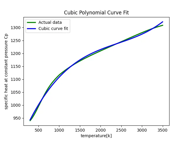
• Depicts the graph plotted for comparison of each linear and cubic fit curves with respect to the original values.
• From the PLOT, it is clear that the cubic fit curve has more accurate value than the linear fit curve.
• To understand more, the error curve gives more idea where it represents the absolute value of error for the two curves at each temperature points.
• It is observed that the cubic curve fit has comparatively lesser error value than other followed by linear.

R-square value for linear and cubic polynomial:

5.How to get the best fit?
Consider the general form for a polynomial of order jj
f(x)=a0+a1x+a2x2+a3x3+...+ajxj=a0+j∑k=0akxkf(x)=a0+a1x+a2x2+a3x3+...+ajxj=a0+∑k=0jakxk

Let this be the equation for the curve fit. The curve that gives minimum error between data yy and the fit f(x)f(x) is the best fit.

The best fit can be obtained by increasing the order of the polynomial and also by splitting the curves into multiple range and then plotting for each range set.

There are different methods to understand the goodness of the curve fit, namely,

1.The sum of squares due to error (SSE), R-square,

2.Adjusted R-square and Root mean squared error (RMSE).

From these quantities, we can evaluate the best fit of the curve.

6.What could be done to improve the cubic fit?
For improving the cubic fit, the splitwise method can be used where the data set in divided into multiple range. More the division, more will be the improvement to the curve.

Conclusion:

By observing the R squared value for each fit, we can say that the splitwise method with cubic function provides the best fit for the given set of data whereas the linear function provided the worst fit.