Week 5 - Curve fitting

1, popt - An array of optimal values for the parameters which minimizes the sum of square of residuals

pcov - 2d array which contains the estimated covariance of popt. The diagonals provide the variance of the parameter estimate.

2, np.array - Converts the python list of temperature into a numpy array where operations like pow are allowed on numpy array, which is not allowed in python list.

3, *popt represents the value stored in array popt.

4, for linear polynomial

code -

import numpy as np 
import matplotlib.pyplot as plt 
from scipy.optimize import curve_fit

 #curve fit function
def func(t,a,b,c,d,e):
 	return a*t+b

 #reading thermodynamic  data file
def read_file():
    temperature=[]
    cp=[]
    for line in open ('data','r'):
         values =line.split(',')
         temperature.append(float(values[0]))
         cp.append(float(values[1]))
        
    return [temperature,cp]

 # main program
temperature, cp=read_file()
popt,pcov=curve_fit(func,temperature,cp)
fit_cp=func(np.array(temperature),*popt)

plt.plot(temperature,cp,color="blue",linewidth=3)
plt.plot(temperature,fit_cp,color="red",linewidth=3)
plt.legend(['actual data','curve fit'])
plt.xlabel('Temperature[K]')
plt.ylabel('Cp')

plt.show()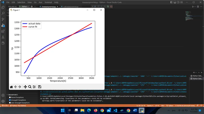

conclusion -

importing numpy, matplotlib.pyplot & scipy modules for mathematical , plotting purposes.

then the defining the required functions & returning its value using return function.

defining a function to the read the file 'data' using def read_file() & creating empty array for temperature & cp

created for loop 7 using 'data' and using append function providing data after every for loop into temperature & cp empty array using return function .

using popt & pcov function creating the curve fit between temperature & cp

then plotting a graph of the actual data between temperature & cp in blue colour with line width 3 & plotting the curve fit between temperature & cp in red colour with line width 3.

also providing xlabel, ylabel, legend & using plt.show() displaying the output graph

for cubical polynomial

code -

import numpy as np 
import matplotlib.pyplot as plt 
from scipy.optimize import curve_fit

 #curve fit function
def func(t,a,b,c,d):
  return a*pow(t,3)+b*pow(t,2)+c*t+d

 #reading thermodynamic data file
def read_file():
    temperature=[]
    cp=[]

    for line in open ('data','r'):
        values =line.split(",")
        temperature.append(float(values[0]))
        cp.append(float(values[1]))

    return [temperature,cp]

 # main program
temperature, cp=read_file()
popt,pcov=curve_fit(func,temperature,cp)
fit_cp=func(np.array(temperature),*popt)

plt.plot(temperature,cp,color="blue",linewidth=3)
plt.plot(temperature,fit_cp,color="red",linewidth=3)
plt.legend(['actual data','curve fit'])
plt.xlabel('Temperature[K]')
plt.ylabel('Cp')

plt.show()

conclusion -

importing numpy, matplotlib.pyplot & scipy modules for mathematical , plotting purposes.

then the defining the required functions & returning its value using return function.

defining a function to the read the file 'data' using def read_file() & creating empty array for temperature & cp

created for loop 7 using 'data' and using append function providing data after every for loop into temperature & cp empty array using return function .

using popt & pcov function creating the curve fit between temperature & cp

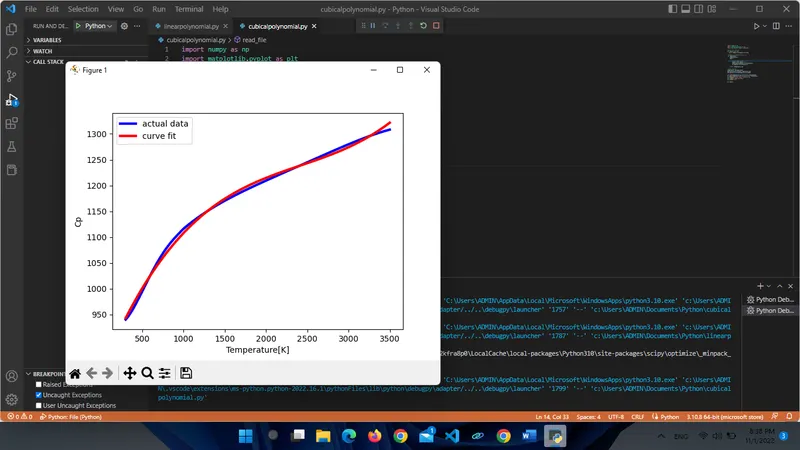
then plotting a graph of the actual data between temperature & cp in blue colour with line width 3 & plotting the curve fit between temperature & cp in red colour with line width 3.

also providing xlabel, ylabel, legend & using plt.show() displaying the output graph

5,

By increasing the degree of the curve we can make the best curve fit.

increasing the degree of the curve to 4, the curve will be more accurate than the cubic polynomial.

increasing the degree of polynomial will increase the complications and time required, hence 4th order polynomial can be taken as a sufficient curve fit.