Week 3 - Solving second order ODEs
this is a ordinary differential equation and trying to write a program in python and creation a nimation file using the graphs
where g = gravity in m/s2, L = length of the pendulum in m, m = mass of the ball in kg, b=damping coefficient. L=1 metre, m=1 kg, b=0.05. g=9.81 m/s2. Simulate the motion between 0-20 sec, for angular displacement=0,angular velocity=3 rad/sec at time t=0.
code -
import math
import matplotlib.pyplot as plt
import numpy as np
from scipy.integrate import odeint

def mode1(theeta, t, b, g, l, m):                        # defining variables

    theeta1 = theeta[0]
    theeta2 = theeta[1]
    dtheeta1_dt = theeta2
    dtheeta2_dt = -(b/m) * theeta2 - (g/l) * math.sin(theeta1)
    dtheeta_dt = [dtheeta1_dt, dtheeta2_dt]
    return dtheeta_dt

b = 0.05
g = 9.81
l = 1
m = 1

# initial condition
theeta_0 = [math.pi/2,3]

# time points taken betaween 0 to 20 with 150 intervals
t = np.linspace(0,20,150)

# solve ode
theeta = odeint(mode1,theeta_0,t,args=(b, g, l, m))

#plotting
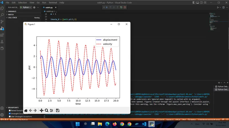
plt.plot(t,theeta[:,0],'b',label=r'$displacment$')
plt.plot(t,theeta[:,1],'r--',label=r'$velocity$')
plt.ylabel('plot')
plt.xlabel('time')
plt.legend(loc='best')
plt.show()

#providing intial points in x & y axis as x0 & y0 respectively, & giving counter variable
P = theeta[:,0]
B = 1
x0 = 0
y0 = 0

#calculating  at different intervals  using foor loop
for i in P:
    x1 = x0 + (l * math.sin(i))
    y1 = y0 - (l * math.cos(i))
    B = B + 1
    filename = str(B) + 'png'

# plotting the co-ordinates & saving and stitching together for animation
    plt.figure()
    plt.plot([-2,2],[0,0],'b-',linewidth=2)
    plt.plot([x0,x1],[y0,y1])
    plt.plot(x1,y1,'o',markersize = 20)
    plt.xlim([-2,2])
    plt.ylim([-2,2])
    plt.title('pendulum')
    plt.savefig(filename)
simple pendulum animation youtube link
graph plotted -

conclusion -
imported modules like math for calculation purpose, matplotlib.pyplot for plotting, numpy for calculating arrays , scipy.integrate for solving differential equations.
intialised and defined variables like theeta, t, b, g, l, m
then the provided second order differential equation is splitted to 2 different first order differential equations. by using
theeta1 = theeta
dtheeta1/dt = theeta2 & dtheeta2/dt = (-b/m) theeta2 - (g/l) sin theata1
where g = gravity in m/s2, l = length of the pendulum in m, m = mass of the ball in kg, b=damping coefficient. l=1 metre, m=1 kg, b=0.05. g=9.81 m/s2.
then intiallising the conditions to theeta_0 where pi/2 for displacement and 0 for velocity
then creating time array linspace from numpy module which is created between 0 to 20 seconds with 150 intervals.
then using odeint from scipy modules to calculate the ordinary differential equation and passing all the argument values to mode 1 where the differential are provided and giving this to equations values to dtheeta_dt using return function
this odeint function use a time an integrates the equation and returns the value & continously integrates it
in plotting (t,theeta[:,0] plots for first ode dtheeta1_dt which is displacement