Week 5 - Curve fitting

1. popt: Creates an array of optimal values for the parameters which minimizes the sum of squars of the residuals.

pcov: Creates a 2D array which contains the estimated covariance of the array created by popt.

2. np.array(temperature) converts the temperature list present in the data file to numpy array on which mathematical operations are performed.

3. The asterisk (*) in *popt means referring to values in the array created by/stored in popt

4. Code:

import numpy as np
import matplotlib.pyplot as plt
from scipy.optimize import curve_fit
def func_linear(t,a,b):
    return a*t+b
def read_file():
    temperature = []
    cp = []
    for line in open('data','r'):
        values = line.split(',')
        temperature.append(float(values[0]))
        cp.append(float(values[1]))
    return [temperature,cp]
temperature,cp = read_file()
popt,pcov = curve_fit(func_linear,temperature,cp)
fit_cp = func_linear(np.array(temperature),*popt)
plt.figure()
plt.plot(temperature,cp,color = 'blue',linewidth = 3)
plt.plot(temperature,fit_cp,color = 'red',linewidth = 3)
plt.title("Specific Heat vs Temperature")
plt.legend(["Actual Data","Curve Fit"])
plt.xlabel("Temperature (in K)")
plt.ylabel("Specific Heat (in KJ/kg.K)")
plt.show()

import numpy as np
import matplotlib.pyplot as plt
from scipy.optimize import curve_fit
def func_cubic(t,a,b,c,d):
    return a*pow(t,3)+b*pow(t,2)+c*t+d
def read_file():
    temperature = []
    cp = []
    for line in open('data','r'):
        values = line.split(',')
        temperature.append(float(values[0]))
        cp.append(float(values[1]))
    return[temperature,cp]
temperature,cp = read_file()
popt,pcov = curve_fit(func_cubic,temperature,cp)
fit_cp = func_cubic(np.array(temperature),*popt)
plt.figure()
plt.plot(temperature,cp,color = 'blue',linewidth = 3)
plt.plot(temperature,fit_cp,color = 'red',linewidth = 3)
plt.title("Specific Heat vs Temperature")
plt.legend(["Actual Data","Curve Fit"])
plt.xlabel("Temperature (in K)")
plt.ylabel("Specific Heat (in KJ/kg.K)")
plt.show()

PROCEDURE FOR THE CODE:

• Import 'numpy', 'matplotlib.pyplot' as 'np' and 'plt' respectively and 'curve_fit' from 'scipy.optimize'.
• Define the linear function as 'func_linear', declare the required variables and give the expresson for obtaining a result.
• Define the function 'read_file' and give the arrays present in the file that has to be read by the program.
• By using the 'for' command, give the conditions required to separate the temperature and cp values.
• Use the 'popt','pcov' and 'curve_fit' commands to obtain the curvefit data for the given temperature and cp values.
• Obtain the curvefitted cp values by converting the temperature values into an numpy array and referring valuesfrom the popt array. Use these obtained values and the temperature array in the 'func_linear' function.
• Plot the graphs of the actual data and curvefitted data with the obtained values by giving the color as blue and red respectively, using 'plt.plot' command.
• Give the title, label the x and y axes and mention the legend in the graph by using 'plt.title','plt.xlabel','plt.ylabel' and 'plt.legend' respectively.
• Repeat the same process for cubic method, but declare an extra variable in the function for the cubic polynomial.

RESULTS:

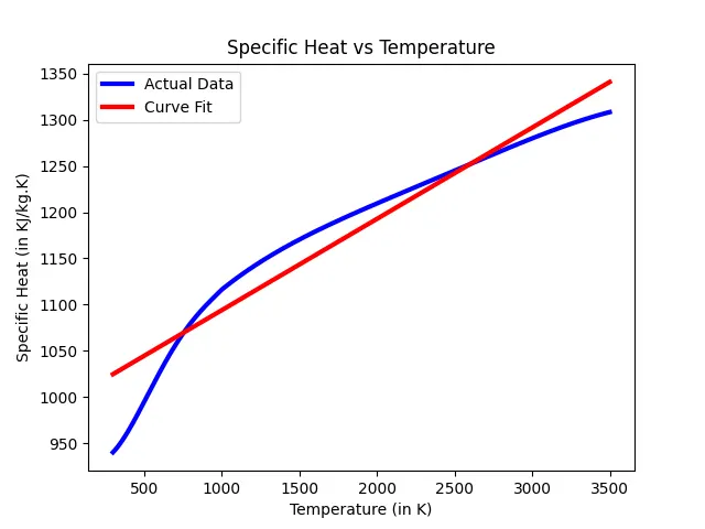
Linear Curve-Fit

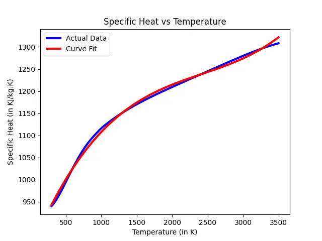
Cubic Curve-Fit

5. The curve is almost fitted perfectely for the cubic polynomial, as shown in the above results. To obtain a perfect fit, we can increase the degree of the polynomial, which would result in much complex calculations and much accurate results.