Week 5 - Curve fitting
Questions and Answer:
1. What does popt and pcov mean?
A: 'popt': It is an array of the coefficients of a polynomial specified at the beginning of the program.
'pcov': It is a square matrix that contains the true variance and covariance of the parameters.
2. What does np.array(temperature) do?
A: Creates an array of temperatures from the values stored ina data file using numpy module.
3. What does the * in *popt mean?
A: It helps to refer to the coefficients of the polynomial into consideration.
4. What needs to be done in order to make the curve fit perfect?
A: To make the curve fit perfect, the value of RMSE should be minimum and the value pf R-square should be close to 1. It can be done by increasing the order of polynomial that we are trying to curve fit.
Aim: To perform curve fitting for the given Temperature and Cp Data in Python.
Theory: Curve fitting is the process of constructing a curve, or mathematical function, that has the best fit to a series of data points, possibly subject to constraints. Curve fitting can involve either interpolation, where an exact fit to the data is required, or smoothing, in which a 'smooth' function is constructed that approximately fits the data. it examines the relationship between one or more predictors (independent variables) and a response variable (dependent variables), with the goal of defining the 'best fit' model of the relationship.
How to choose the best fit?
Upon finding a curve that satisfies the data points there are 4 quantities that help us measure the goodness of fit criteria or how well the equation is representing the data points. They are listed as:
- The sum of squares due to error (SSE)
- R-square
- Adjusted R-Square
- Root Mean Square Error (RMSE)
How to get the best fit?
A line of best fit can be roughly determined using an eyeball method by drawing a straight line on a scatter plot so that the number of points above the line and below the line is about equal (and the line passes through as many points as possible).
Also, the Split Polynomial technique can be opted to obtain a curve fit closest to the data set. this is one of the most viable techniques to perform for the best fit.
What could be done to improve the cubic fit?
- Increase the number of iterations or function evaluations allowed.
- Reduce the convergence tolerance.
- Try also sub-setting the data and fitting different subsets of data separately.
Governing Equations:
1. Sum of Squares Total (SST) – The sum of squared differences between individual data points (yi) and the mean of the response variable (y).
2. Sum of Squares Regression (SSR) – The sum of squared differences between predicted data points (ŷi) and the mean of the response variable(y).
3. Sum of Squares Error (SSE) – The sum of squared differences between predicted data points (ŷi) and observed data points (yi).

The following relationship exists between these three measures:
SST = SSR + SSE
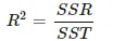
4. SSR, SST and R-Squared - R-squared sometimes referred to as the coefficient of determination, is a measure of how well a linear regression model fits a dataset. It represents the proportion of the variance in the response variable that can be explained by the predictor variable.
The value for R-squared can range from 0 to 1. A value of 0 indicates that the response variable cannot be explained by the predictor variable at all. A value of 1 indicates that the response variable can be perfectly explained without error by the predictor variable.
Using SSR and SST, we can calculate R-squared as:
5. Adjusted R-Squared
The relationship between R Squared and degrees of freedom is that R Squared will always increase as the degrees of freedom decrease which as we saw earlier drastically reduces the reliability of the model. Adjusted R Squared, however, makes use of the degree of freedom to compensate and penalize for the inclusion of a bad variable. Adjusted R Squared can be expressed as :
i.e.
Where,
- k is the number of independent variables
- n is the number of observations
The value of Adjusted R Squared decreases as k increases also while considering R Squared acting as a penalization factor for a bad variable and a rewarding factor for a good or significant variable. Adjusted R Squared is thus a better model evaluator and can correlate the variables more efficiently than R Squared.
6. Root Mean Square Error (RMSE)
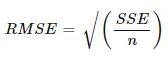
The Root Mean Square Error or RMSE is a frequently applied measure of the differences between numbers (population values and samples) which is predicted by an estimator or a mode. The RMSE describes the sample standard deviation of the differences between the predicted and observed values. Each of these differences is known as residuals when the calculations are done over the data sample that was used to estimate, and known as prediction errors when calculated out of sample. The RMSE aggregates the magnitudes of the errors in predicting different times into a single measure of predictive power.
Objective:
- Curve Fitting of the Temperature and Cp
- Determining Goodness of fit.
Inputs:
Data file (Temperature vs Cp): https://drive.google.com/file/d/1vWi9Vj3AdQf0gqUK1u9jwS8zg92BHGR0/view
Python Program:
# To measure fitness characteristics of the linear and cubic polynomial for the Cp data

import math
import matplotlib.pyplot as plt
import numpy as np
from scipy.optimize import curve_fit

# Curve fit function
# Linear function
def function_1(t,a,b):
	return a * t + b


# Quadratic function
def function_2(t,a,b,c):
	return a * pow(t,2) + b * t + c


# Cubic function
def function_3(t,a,b,c,d):
	return a * pow(t,3) + b * pow(t,2) + c * t + d


# Biquadratic function
def function_4(t,a,b,c,d,e):
	return a * pow(t,4) + b * pow(t,3) + c * pow(t,2) + d * t + e

# Reading thermodynamic data file

def read_file():
	temperature = []
	cp = []
	for line in open('data','r'):
		values = line.split(',')
		temperature.append(float(values[0]))
		cp.append(float(values[1]))

	return [temperature , cp]

# Main Program
temperature , cp = read_file()

# Linear Curve-fit
popt, pcov = curve_fit(function_1,temperature,cp)
fit_cp_l = function_1(np.array(temperature), *popt)

# Plotting graph
plt.figure(1)
plt.plot(temperature,cp,'k--')
plt.plot(temperature,fit_cp_l,color='red',linewidth = 1)
plt.legend(['Actual Data','Curve-fit Data'])
plt.xlabel('Temperature (K)')
plt.ylabel('Cp')
plt.title('Linear Curve Fitting')
plt.grid()
plt.savefig('Linear Curve')
plt.show()

# Quadratic Curve-fit
popt, pcov = curve_fit(function_2,temperature,cp)
fit_cp_q = function_2(np.array(temperature), *popt)

# Plotting graph
plt.figure(2)
plt.plot(temperature,cp,'k--')
plt.plot(temperature,fit_cp_q,color='red',linewidth = 1)
plt.legend(['Actual Data','Curve-fit Data'])
plt.xlabel('Temperature (K)')
plt.ylabel('Cp')
plt.title('Quadratic Curve Fitting')
plt.grid()
plt.savefig('Quadratic Curve')
plt.show()

# Cubic Curve-fit
popt, pcov = curve_fit(function_3,temperature,cp)
fit_cp_c = function_3(np.array(temperature), *popt)

# Plotting graph
plt.figure(3)
plt.plot(temperature,cp,'k--')
plt.plot(temperature,fit_cp_c,color='red',linewidth = 1)
plt.legend(['Actual Data','Curve-fit Data'])
plt.xlabel('Temperature (K)')
plt.ylabel('Cp')
plt.title('Cubic Curve Fitting')
plt.grid()
plt.savefig('Cubic Curve')
plt.show()

# Biquadratic Curve-fit
popt, pcov = curve_fit(function_4,temperature,cp)
fit_cp_b = function_4(np.array(temperature), *popt)

# Plotting graph
plt.figure(4)
plt.plot(temperature,cp,'k--')
plt.plot(temperature,fit_cp_b,color='red',linewidth = 1)
plt.legend(['Actual Data','Curve-fit Data'])
plt.xlabel('Temperature (K)')
plt.ylabel('Cp')
plt.title('Biquadratic Curve Fitting')
plt.grid()
plt.savefig('Biquadratic Curve')
plt.show()

'''
Measuring the fitness characteristics of the curves

SSE (sum of squared Error)
SSR (sum of squares of the Regression)
SST = SSE + SSR (sum of squares Total)
R^2 = SSR/SSE  (R-square)
RMSE = (SSE/l)^0.5 (Root Mean Square Error)

Finding the mean of Cp data
mean = ( Sum of all elements) / (Total number of elements)
'''

s = np.sum(cp)  # Sum of all elements
l = np.size(cp) # Total number of elements
m = s / l       # Mean of Cp data
print('Mean of all Cp: ',m)
print('\n')

# For Linear Curve-fit
linear_sse = 0
linear_ssr = 0
for i in range(l):
	linear_error = abs((np.sum((cp[i] - fit_cp_l[i]))))
	linear_sse = linear_sse + pow(linear_error,2)
	linear_ssr = linear_ssr + np.sum(pow((fit_cp_l[i] - m),2))

print('Fitness Charateristics of the Linear Curve-fit')
linear_sst = linear_sse + linear_ssr
print('linear_sst: ',linear_sst)
linear_R2 = linear_ssr / linear_sst
print('linear_R2: ',linear_R2)
linear_rmse = pow((linear_sse/l),0.5)
print('linear_rmse: ',linear_rmse)
print('\n')

# For Quadratic Curve-fit
quad_sse = 0
quad_ssr = 0
for i in range(l):
	quad_error = abs((np.sum((cp[i] - fit_cp_q[i]))))
	quad_sse = quad_sse + pow(quad_error,2)
	quad_ssr = quad_ssr + np.sum(pow((fit_cp_q[i] - m),2))

print('Fitness Charateristics of the Quadratic Curve-fit')
quad_sst = quad_sse + quad_ssr
print('quad_sst: ',quad_sst)
quad_R2 = quad_ssr / quad_sst
print('quad_R2: ',quad_R2)
quad_rmse = pow((quad_sse/l),0.5)
print('quad_rmse: ',quad_rmse)
print('\n')

# For Cubic Curve-fit
cubic_sse = 0
cubic_ssr = 0
for i in range(l):
	cubic_error = abs((np.sum((cp[i] - fit_cp_c[i]))))
	cubic_sse = cubic_sse + pow(cubic_error,2)
	cubic_ssr = cubic_ssr + np.sum(pow((fit_cp_c[i] - m),2))

print('Fitness Charateristics of the Cubic Curve-fit')
cubic_sst = cubic_sse + cubic_ssr
print('cubic_sst: ',cubic_sst)
cubic_R2 = cubic_ssr / cubic_sst
print('cubic_R2: ',cubic_R2)
cubic_rmse = pow((cubic_sse/l),0.5)
print('cubic_rmse: ',cubic_rmse)
print('\n')

# For Biquadratic Curve-fit
biquad_sse = 0
biquad_ssr = 0
for i in range(l):
	biquad_error = abs((np.sum((cp[i] - fit_cp_b[i]))))
	biquad_sse = biquad_sse + pow(biquad_error,2)
	biquad_ssr = biquad_ssr + np.sum(pow((fit_cp_b[i] - m),2))

print('Fitness Charateristics of the Biquadratic Curve-fit')
biquad_sst = biquad_sse + biquad_ssr
print('biquad_sst: ',biquad_sst)
biquad_R2 = biquad_ssr / biquad_sst
print('biquad_R2: ',biquad_R2)
biquad_rmse = pow((biquad_sse/l),0.5)
print('biquad_rmse: ',biquad_rmse)
print('\n')
Explanation of Program:
1. Initially, the necessary modules are imported and the required functions are specified.
2. A function for reading the data file provided is aiso written and arrays are formed for temperature and Cp values.
3. The linear curve fit it initiated using popt and pcov commands.
4. The curve fitted graphs are lotted with legends and comparison is done.
5. Similarly, curve fit is initiated for Quadratic, cubic, and Biquadratic polynomials.
6. The best fit is chosen and the limitations are mentioned using the 'Goodness o Fit' criterion.
7. The SST, RMSE, and R-SQUARE Values are cal ulated and the results are mentioned for comparison purposes.
Results:
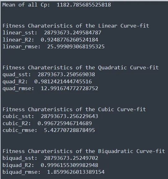
The values of SST, RMSE and R-square are mentioned in the command window.
Plots:
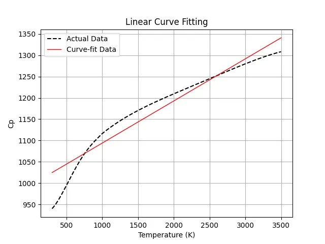
The Linear fit doesn't satisfy the purpose and higher-order polynomial should be considered.
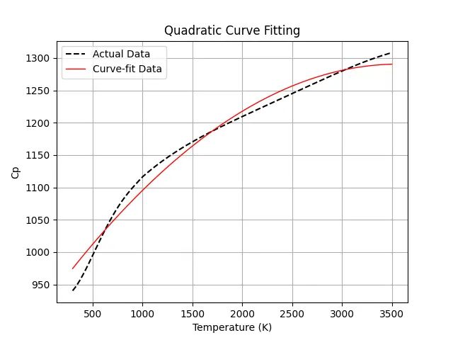
The blueprint comes out to be satisfactory but the accuracy of the fit is highly poor.
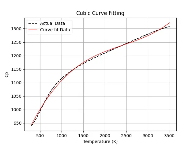
The above fit shows high accuracy but for a perfect fit, the order of the polynomial should be increased.
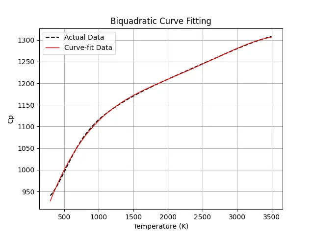
The results are highly accurate and the value of RMSE is least for Biquadratic Curve Fit. Also, the value of R-square is closest to 1.
Error:
The below figure shows the error encountered while programming i.e., I have not defined the values for Cp. So it is showing 'ydata' must not be empty!
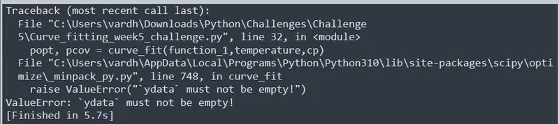
It is corrected by defining the values pf Cp.
Conclusion:
Curve fitting of the given data by suitable methods and techniques in order to produce the best fit. The goodness of fit measure is satisfied by calculating variables of interest. The Linear Fit curve doesn't satisfy the criterion whereas Biquadratic Curve satisfies it.