Challenge

Week 5 - Curve fitting

SSikkandar Faiz17 Apr 2022

main code for linear curve fit:

#importing the required modules for the function to understand the input modules
import numpy as np
import matplotlib.pyplot as plt
from scipy.optimize import curve_fit

#here we are to make a linear regression curve fit the given data.
#since it is for a linear curve 3 inputs are taken for the function.
def func(t, a, b):

	#it is of format ax+b

	return ((a*t) + b)

#the function unpacks the data from the storage directory and states them to their respective variable.
def read_file():
	#the values of the temperature from the data if stored here.
	temperature = []
	#the values of the specific heat from the data if stored here.
	cp = []
	#it helps in unpack data
	for line in open('data','r'):
		values = line.split(',')
		temperature.append(float(values[0]))
		cp.append(float(values[1]))
	#the values of temperature and specific heat are then taken to their respective arrays with return command
	return [temperature,cp]

#the variables temperature and specific heat are then taken from the function and into the curve fit command for the solution.
temperature, cp = read_file()
#curve fit is formulated with the given variables.
popt, pcov = curve_fit(func, temperature, cp)
fit_cp_li = func(np.array(temperature),*popt)


#plotting of the main data and the curve fit data is done for better understanding of the results.
plt.plot(temperature,cp,color = 'b',linewidth = 6)
plt.plot(temperature,fit_cp_li,color ='r',linewidth = 3)
plt.legend(['real data','curve fit'])
plt.xlabel('temperature')
plt.ylabel('cp')
plt.show()


#goodness of fit
s = np.sum(cp)
l = np.size(cp)
m = s/l #finding mean
print('mean of cp : ', m)
print('') #line gap

#for linear curve fit
lin_sse = 0
lin_ssr = 0 
for i in range(l):
	lin_error = abs((np.sum((cp[i] - fit_cp_li[i]))))
	lin_sse = lin_sse+pow(lin_error,2)
	lin_ssr = lin_ssr + np.sum(pow((fit_cp_li[i] - m),2))

#the values are calculated for linear_sst, linear_R2, linear_RMSE.
print('for linear curve fit')
lin_sst = lin_sse+lin_ssr
print('linear_sst : ',lin_sst)
lin_r2 = lin_ssr/lin_sst
print('linear_R2 : ', lin_r2)
lin_rmse = pow((lin_sse/l),0.5)
print('linear_RMSE : ', lin_rmse)
print('')

plot for the fit:

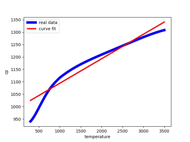
we can see the real data curve is not well traced by the linear curve.

explanation for the code:

required modules are imported from the library.

#importing the required modules for the function to understand the input modules

import numpy as np
import matplotlib.pyplot as plt
from scipy.optimize import curve_fit

in the linear cubic fit we are taking in a linear polynomial equation, which is in the format ax+b.

#here we are to make a linear regression curve fit the given data.

#since it is for a linear curve 3 inputs are taken for the function.

def func(t, a, b):

#it is of format ax+b

return ((a*t) + b)

the function unpacks the data from the storage directory and states them to their respective variable.

def read_file():

the values of the temperature from the data if stored here.

temperature = []

the values of the specific heat from the data if stored here.

cp = []

for loop helps in unpacking data and assigning them to their own respective variables.
for line in open('data','r'):
values = line.split(',')
temperature.append(float(values[0]))
cp.append(float(values[1]))

the values of temperature and specific heat are then taken to their respective arrays with return command

return [temperature,cp]

the variables temperature and specific heat are then taken from the function and into the curve fit command for the solution.

temperature, cp = read_file()

curve fit is formulated with the given variables.

popt, pcov = curve_fit(func, temperature, cp)
fit_cp_li = func(np.array(temperature),*popt)

plotting of the main data and the curve fit data is done for better understanding of the results.
plt.plot(temperature,cp,color = 'b',linewidth = 6)
plt.plot(temperature,fit_cp_li,color ='r',linewidth = 3)
plt.legend(['real data','curve fit'])
plt.xlabel('temperature')
plt.ylabel('cp')
plt.show()

goodness of fit is calculated to show how well the fit is.
s = np.sum(cp)
l = np.size(cp)
m = s/l #finding mean
print('mean of cp : ', m)
print('') #line gap

for linear curve fit the basic required variables to solve the sse, r2, rmse values are stated.
lin_sse = 0
lin_ssr = 0
for i in range(l):
lin_error = abs((np.sum((cp[i] - fit_cp_li[i]))))
lin_sse = lin_sse+pow(lin_error,2)
lin_ssr = lin_ssr + np.sum(pow((fit_cp_li[i] - m),2))

#the values are calculated for linear_sst, linear_R2, linear_RMSE.
print('for linear curve fit')
lin_sst = lin_sse+lin_ssr
print('linear_sst : ',lin_sst)
lin_r2 = lin_ssr/lin_sst
print('linear_R2 : ', lin_r2)
lin_rmse = pow((lin_sse/l),0.5)
print('linear_RMSE : ', lin_rmse)
print('') #gap for the line

------------------------------------------------------------------------------------------------------------------------------------------------------------------------------------------------------------------------------------------------------------------------------------------

code for cubic fit:

#importing the required modules for the function to understand the input modules
import numpy as np
import matplotlib.pyplot as plt
from scipy.optimize import curve_fit

#here we are to make a cubic regression curve fit the given data.
#since it is for a cubic curve 5 inputs are taken for the function.
def func(t, a, b, c, d):
	
	#it is of format ax³+bx²+cx+d
	
	return a*pow(t,3) +  b*pow(t,2) +  c*t + d

#the function unpacks the data from the storage directory and states them to their respective variable.
def read_file():
	#the values of the temperature from the data if stored here.
	temperature = []
	#the values of the specific heat from the data if stored here.
	cp = []
	#it helps in unpack data
	for line in open('data','r'):
		values = line.split(',')
		temperature.append(float(values[0]))
		cp.append(float(values[1]))

	#the values of temperature and specific heat are then taken to their respective arrays with return command
	return [temperature,cp]


#the variables temperature and specific heat are then taken from the function and into the curve fit command for the solution.
temperature, cp = read_file()
#curve fit is formulated with the given variables.
popt, pcov = curve_fit(func, temperature, cp)
fit_cp_cu = func(np.array(temperature),*popt)

#plotting of the main data and the curve fit data is done for better understanding of the results.
plt.plot(temperature,cp,color = 'b',linewidth = 6)
plt.plot(temperature,fit_cp_cu,color ='r',linewidth = 3)
plt.legend(['real data','curve fit'])
plt.xlabel('temperature')
plt.ylabel('cp')
plt.show()


#goodness of fit
s = np.sum(cp)
l = np.size(cp)
m = s/l #finding mean
print('mean of cp : ', m)
print('') #line gap

#for cubic curve fit
cub_sse = 0
cub_ssr = 0 
for i in range(l):
	cub_error = abs((np.sum((cp[i] - fit_cp_cu[i]))))
	cub_sse = cub_sse+pow(cub_error,2)
	cub_ssr = cub_ssr + np.sum(pow((fit_cp_cu[i] - m),2))

#the values are calculated for cubic_sst, cubic_R2, cubic_RMSE.
print('for cubic curve fit')
cub_sst = cub_sse+cub_ssr
print('cubic_sst : ',cub_sst)
cub_r2 = cub_ssr/cub_sst
print('cubic_R2 : ', cub_r2)
cub_rmse = pow((cub_sse/l),0.5)
print('cubic_RMSE : ', cub_rmse)
print('')

plot for cubic:

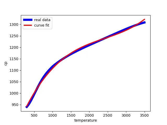
we can see that when we take in higher order polynomial equation the curve fit we make traces the real data much good.

explanation of the code:

everything is similar to linear curve fit, except the polynomial data made as the input.

here since it is for cubic fit we are to take a third order polynomial so we are to derive the code for t, a, b, c, d in the format of ax³+bx²+cx+d.

which becomes a*pow(t,3) + b*pow(t,2) + c*t + d

split wise code for the curve fit:

#importing the required modules for the function to understand the input modules
import numpy as np
import matplotlib.pyplot as plt
from scipy.optimize import curve_fit

#the function unpacks the data from the storage directory and states them to their respective variable.
def read_file():
	#the values of the temperature from the data if stored here.
	temperature = []
	#the values of the specific heat from the data if stored here.
	cp = []

	#it helps in unpack data
	

	for line in open('data','r'):
		values = line.split(',')
		temperature.append(float(values[0]))
		cp.append(float(values[1]))
		
	#the values of temperature and specific heat are then taken to their respective arrays with return command
	return [temperature,cp]

#the variables temperature and specific heat are then taken from the function and into the curve fit command for the solution.
temperature, cp = read_file()
#the values of the temperature and specific heat data are divided into four as we are doing  split wise method.every thing is same as the cubic but the temperature and the cp values are taken as four different vaariable inputs.
temperature_1 = temperature[0:800]
temperature_2 = temperature[800:1600]
temperature_3 = temperature[1600:2400]
temperature_4 = temperature[2400:3200]
cp1 = cp[0:800]
cp2 = cp[800:1600]
cp3 = cp[1600:2400]
cp4 = cp[2400:3200]


#here we are to make a cubic regression curve fit the given data.
#since it is for a cubic curve 5 inputs are taken for the function.
def func(t, a, b, c, d):

	#it is of format ax³+bx²+cx+d

	return a*pow(t,3) +  b*pow(t,2) +  c*t + d


#curve fit is formulated with the given variables for the given data temperature and specific heat.
popt, pcov = curve_fit(func,temperature, cp)
fit_cp_cu = func(np.array(temperature),*popt)


#curve fit is formulated with the given variables for the first set of temperature and specific heat data of the curve fit.
popt1, pcov1 = curve_fit(func,temperature_1, cp1)
fit_cp_cu1 = func(np.array(temperature_1),*popt1)

#curve fit is formulated with the given variables for the second set of temperature and specific heat data of the curve fit.
popt2, pcov2 = curve_fit(func,temperature_2, cp2)
fit_cp_cu2 = func(np.array(temperature_2),*popt2)

#curve fit is formulated with the given variables for the third set of temperature and specific heat data of the curve fit.
popt3, pcov3 = curve_fit(func,temperature_3, cp3)
fit_cp_cu3 = func(np.array(temperature_3),*popt3)

#curve fit is formulated with the given variables for the fourth set of temperature and specific heat data of the curve fit.
popt4, pcov4 = curve_fit(func,temperature_4, cp4)
fit_cp_cu4 = func(np.array(temperature_4),*popt4)

#the plotting of the real data is done and the plot for the optimizing curve is made too.
#the plottings are done and the 4 sets of data are made to see their best fit.
plt.plot(temperature,cp,color = 'r',linewidth = 6)
plt.plot(temperature_1,fit_cp_cu1,color = 'b',linewidth = 3)
plt.plot(temperature_2,fit_cp_cu2,color = 'g',linewidth = 3)
plt.plot(temperature_3,fit_cp_cu3,color = 'y',linewidth = 3)
plt.plot(temperature_4,fit_cp_cu4,color = 'c',linewidth = 3)
#labels are done for better understanding.
plt.xlabel('temperature')
plt.ylabel('cp')
plt.show()

plot for split wise cubic curve fit:

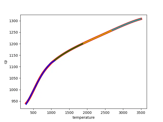
we can see the predicted curve fits the real data much much more perfect than the above single cubic fit.

explanation for the split wise curve fit:

the fit is similar to the cubic fit above, it uses the same polynomial equation. the major change is that the curve we are to trace is split into four different curve than a single curve. by doing such we can make our predicting curve to trace the real data curve much well than the cubic single curve.

the values of good fit is calculated for both the curves:

for linear curve fit:

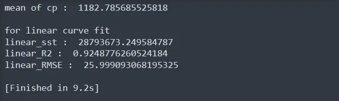
rmse value is much than the cubic fit.

for cubic fit:

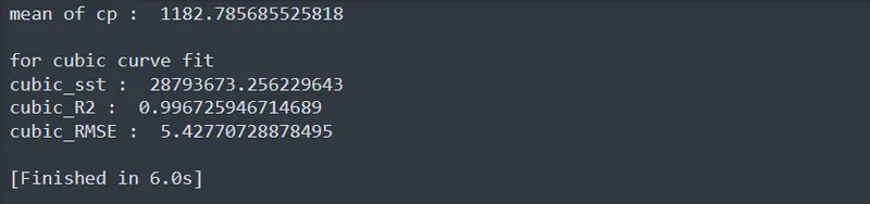
rmse value is reduced than the linear curve fit.

parameters of goodness of fit:

1.sum of squares error (SSE): it represents the gap between the predicted value and the actual value. value closer to 0 indicates a better fit.

SSE = Σ(Y VALUE - VALUE OF Y REGRESSION)^2

2.R squared: R^2 is but the SSR/SST. SSR is but the gap between the mean and the predicted value of y and sst is but the total of sse and ssr. r^2 has values between 0 and 1. it gives how close the data points is to the regression line. if the datas are scattered we can understand we will get alow r^2 value. so if the r^2 value is close to 1, its a good fit.

Root mean square error (RMSE):

sum of the difference between the actual and the predicted data values are taken for all the data points, which then squared and the sum of them is taken followed by average or mean. finally the value is taken square root which is the RMSE. value of rmse close to 0 is good.

QUESTION TO ANSWER:

1.What does popt and pcov mean?

popt is an array that stores the coefficients that are passed onto the function

pcov is a 2 dimentional array which contains the estimated covariance of popt. that is the coefficients of popt.The diagonals provide the variance of the parameter estimate.

2.What does np.array(temperature) do?

the values in the temperature variable is saved into an array format output.

3.What does the * in *popt mean?

it represents the collection of variables of the inputs individually which are stored in the popt.

4.Write code to fit a linear and cubic polynomial for the Cp data. Explain if your results are good or bad.

the codes are executed and the results are plotted and the good and bad conditions are explained below the codes individually.

5.What needs to be done in order to make the curve fit perfect?

by increasing the order of the polynomial equation we can attain a good curve with less deviance from the original data.

6.Show empirically as to how well your curve has been fit.

the curve called split wise fits the real data well and the explanations for it is provided below each plots.

there wasn't much since ive had knowledge of it previously in matlab.

conclusion:

Hope the questions have been answered and the plots are better in showing the outputs.

Week 5 - Curve fitting

Ship work like this
in your own course.

Talk to a career counsellor

Ship work like thisin your own course.

Talk to a career counsellor

Ship work like this
in your own course.