Week 3 - Solving second order ODEs
MAIN CODE :
clear all
close all
clc

% to give in the basic needed inputs
%the gravity as we all know (m/s^2)
g = 9.81;
% damping value for the pendulum
b = 0.05;
% mass of the object (kg)
m = 1;
% length of the pendulum(m)
l = 1;

% value of theta
theta_0 = [0;3];

% initial conditions
t_span = linspace(0,20,500);
%counter
ct = 1;

%ode function
[t, results] = ode45(@(t,theta) ode_func(t, theta, b,g,l,m),t_span, theta_0);

%plotting
figure(1)
plot(t,results(:,1))
hold on
plot(t,results(:,2))
ylabel('velocity and displacement')
xlabel('time')

%creating an animation of the pendulum
%looping to create a perfect environment
holder = results(:,1);
for i = 1:length(holder)
    trace = holder(i);
%the attached end of the pendulum
    x0 = 0;
    y0 = 0;
%the free oscillating end of the pendulum
    x1 = l*sin(trace)
    y1 = -l*cos(trace)
%plotting the pendulum for better understanding
    figure(2)
    plot([-1.5 1.5],[0 0],'color','r','linewidth',6);
    hold on
    plot([x0 x1],[y0 y1],'color','g','linewidth',3);
    hold on
    plot(x1,y1,'o','markers',25,'markerfacecolor','b');
    hold off
    grid on
    axis([-2 2 -2 1]);
    pause(0.05)


    %converting the data collected into a video file
    M(ct) = getframe(gcf);
    ct = ct+1;
end
%editing movie file
movie(M)
videofile = VideoWriter('simple pendulum.avi','uncompressed AVI')
open(videofile)
writeVideo(videofile,M)
close(videofile)
FUNCTION CODE :
function [dtheta_dt] = ode_func(t,theta,b,g,l,m)
 theta1 = theta(1)
 theta2 = theta(2)
 dtheta1_dt = theta2;
 dtheta2_dt = -(b/m)*theta2 - (g/l)*sin(theta1);
 dtheta_dt = [dtheta1_dt; dtheta2_dt];
end
EXPLAINING MAIN CODE :
starting with clear all, close all, clc like all time for better refreshment of the editor to future code.
clear all
close all
clc
the inputs for the function or the code to run successfully to give a better understanding of the second order ode. the motion of a pendulum is a simple example for the second order ode.for a pendulum to be pctured we need the mass of the pendulum which is added as 1kg. the length of the pendulum is added as 1m. the gravitational force acting on the pendulum is made sure to be present as 9.81m/s^2. and the damping force, which is an opposing force that acts in direction opposite to the oscillation of the pendulum.
% to give in the basic needed inputs
%the gravity as we all know (m/s^2)
g = 9.81;
% damping value for the pendulum
b = 0.05;
% mass of the object (kg)
m = 1;
% length of the pendulum(m)
l = 1;
what we speak of here is but the major two values that is the initial displacement of the pendulum and the initial velocity with which the pendulum is released. initial displace ment is kept as 0 as asked and the initial velocity is made to be 3 m/s. theta_0 represents the first value as the initial displacement and the second value as the initial velocity.
% value of theta
theta_0 = [0;3];
here we make the time for which the oscillation of the pendulum is to recorded. the time count is made to be from 0 to 20 with divisions in between as 500 for smother trace of the pendulum when animated.
% initial conditions
t_span = linspace(0,20,500);
counter helps during the convertion of the plots into an animation
%counter
ct = 1;
the main function for the whole second order ode to work is but defined. the fist square brackets represents the values that are to be made as the output once the function on the right is complete. moving on to the right we can see ode45(@(t,theta) which is a matlab inbuilt function which represents that the funtion is to be solved by ode method and has two values time(t) and theta which are the independent and dependent variables. following that we see the input function for the code to work, this function is added to the main code for the ode operations to be held. will explain the input function below seperately.
%ode function
[t, results] = ode45(@(t,theta) ode_func(t, theta, b,g,l,m),t_span, theta_0);
this plotting is to show that the ode funtion has been performed just the way we want to. we mentioned it as figure 1 because we are to make an animation next which is defined as figure 2. first plot here gives the values printed for the displacement and the second for the velocity with respect to time.
%plotting
figure(1)
plot(t,results(:,1))
hold on
plot(t,results(:,2))
ylabel('displacement')
xlabel('time')
we are to create a variable, it can be anything. i named it as holder. it is to hold values from the results(:,1). the reesult(:,1) holds the values of the displacement of the pendulum so we are placing all its values in holder first. then we are creating a variable called i which holds the exact number of values as the holder since we made it to hold matching values as holder. after then we are making the variable called trace which will help in oscillating the pendulum when animated.
%creating an animation of the pendulum
%looping to create a perfect environment
holder = results(:,1);
for i = 1:length(holder)
trace = holder(i);
we are creating the fixed points of the pendulum, naming them as x0 y0.
%the attached end of the pendulum
x0 = 0;
y0 = 0;
here the oscillating ends of the pendulum
%the free oscillating end of the pendulum
x1 = l*sin(trace)
y1 = -l*cos(trace)
ploting of the pendulum for better understanding, we here plot a line ffirst that is the plot from -1.5 to 1.5 this acts as the base from which the pendulum suspends and then the fixed points in it which are x0 and y0. we are marking them in red color and with a width of 6mm. it is followed by hold on for not to be deleted when another plot is made.
%plotting the pendulum for better understanding
figure(2)
plot([-1.5 1.5],[0 0],'color','r','linewidth',6);
hold on
here we are to plot the suspended region of the pendulum. we have named the free end as x1 any y1. we link both the ends of the pendulum with a green line which has a width of 3mm the length is 1m, followed by hold on for the previous reasons.
plot([x0 x1],[y0 y1],'color','g','linewidth',3);
hold on
we are making a mass ball at the bottom of the free end with the marker command. hold is off to make the pendulum trace the plot.
plot(x1,y1,'o','markers',25,'markerfacecolor','b');
hold off
grid on
axis([-2 2 -2 1]);
pause(0.05)
the plots made is then made into a movie with the help of the movie command
%converting the data collected into a video file
M(ct) = getframe(gcf);
ct = ct+1;
end
the videofile is named with an assigned format made to open and to add all the inputs and closed for future reference.
%editing movie file
movie(M)
videofile = VideoWriter('simple pendulum.avi','uncompressed AVI')
open(videofile)
writeVideo(videofile,M)
close(videofile)
EXPLAINING FUNCTION INPUT CODE :
to understand this we are to breakdown the initial second order ode into two first order odes
given ode equation:
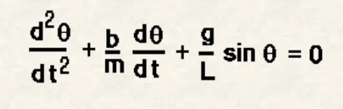
to break it down we assume θ = θ1
substituting this to dθ/dt we will end up having dθ1/dt we assume it as θ2
having this two we make the initial given into
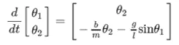
we then consider θ1 and θ2 at first square bracket to be just θ
this whole thing above is the main function formula which is written as below :
function [dtheta_dt] = ode_func(t,theta,b,g,l,m)
theta1 = theta(1)
theta2 = theta(2)
dtheta1_dt = theta2;
dtheta2_dt = -(b/m)*theta2 - (g/l)*sin(theta1);
dtheta_dt = [dtheta1_dt; dtheta2_dt];
end
this is then substituted in the main function for the pendulum animation to obtain.
ERRORS:
1.at first i mentioned the free end points as x1 = l*sind(trace)
y1 = -l*cosd(trace) which made the pendulum oscillate very small since i took them in terms of degree
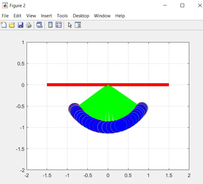
2.forgot to off the hold at the end of the second figure which gave result as
3.forgot to capitalise the w in VideoWrite, which gave output as

ERROR CORRECTION:
1.took away the d at the end of sin and cos, which gave a good amount of oscillation.
2.made the hold command off at the end of the second figure which gave a better oscillating animation.
3.rectified the capital W in VideoWriter, gave right output.
END PLOT :
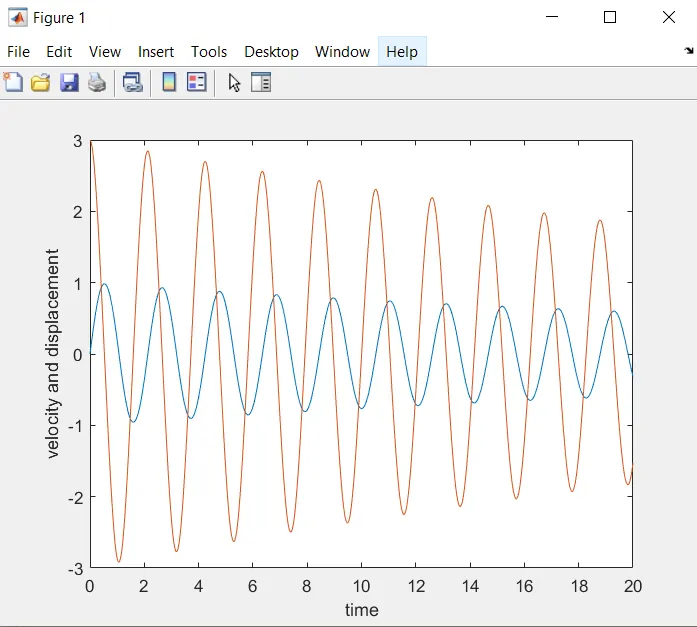
orange line shows the velocity and the blue gives the displacement. we can see as time goes by both the velocity and displacement gradually reduces
ANIMATION :
https://youtu.be/yCRZKEHvGH4