Project 2 - Rankine cycle Simulator
To plot the visualisation of rankine cycle. it is the basic and most effective representation of modern day thermal and nuclear power plants. the working of the rankine cycle is broken down into four process for better understanding. the cycle converts the thermal energy into mechanical energy and then into electrical energy. the system contains water as the working fluid.
picturistic representation of the rankine cycle:
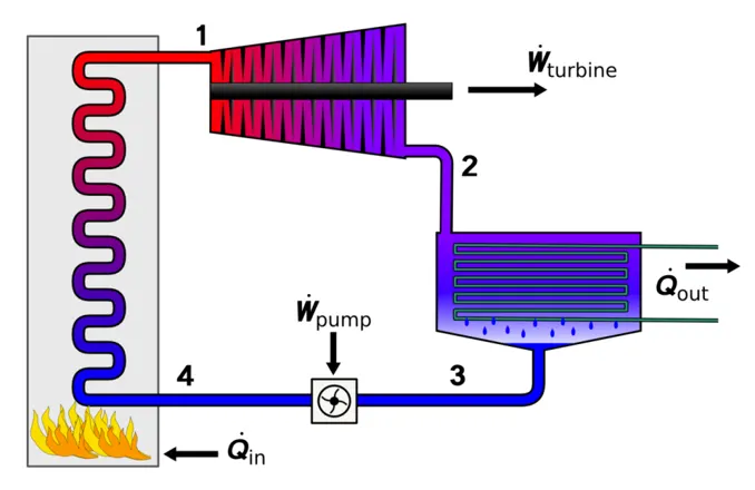
the numbers shows the working of the cycle, that is the way the system works from 1 to 4.
process 1 - 2:
in this process the expanded or heated thermal energy from the boiler is sent into the turbine, where the thermal power makes the turbine rotate which is a mechanical work followed by producing electricity as the turbine is attached to the generator.
process 2 -3:
in this stage the thermal energy after losing its power or effectiveness due to generation of power is sent to the condenser. here cold water is made to circulate in a closed system where the condensation(conversion from gas to liquid) process takesplace.
process 3-4:
in this stage the water from the condenser is again made to enter into the boiler where it can be heated or super heated. the pump helps in achieving the flow of water from condenser to the boiler in a compressed way or as a pressurised fluid.
process 4-1:
here again the water is heated by means of adding heat and it is then made to rush with high pressure into the turbine.
wt is the turbine output, that is the energy or work output due to the rotation.
Qout is the thermal heat that is taken out of the water or gas in the condenser.
wpump is water pump
Qin is the heat added.
EQUATIONS:
the efficiency of rankine cycle is wrtten as:
Ntherm = [(Work Output — Work input)/Heat entered into the system].
the work done by pump is equal to 1% of total turbine output so it can be neglected.
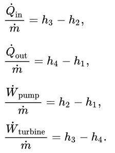
when dealing eff of turbine and pump some changes has to be done:

variables:
Q = heat flow of the system.
w = mechanical work of the system.
m = mass flow of the system.
ntherm = thermal effiiency of the system.
h1,h2,h3,h4 are the enthalpies at four stages.
p1 and p2 are pressure before and after compression.
MAIN CODE:
clear all
close all
clc
%display
disp('Rankine cycle simulator');
disp('1-2 isentropic expansion in the turbine')
disp('2-3 constant pressure heat rejection by condenser')
disp('3-4 isentropic compression in the pump')
disp('4-1 constant pressure heat addition by boiler')

%required inputs
t_1 = input('temperature at turbine inlet(in degree celcius): ');
p_1 = input('pressure at turbine inlet(in bar): ');
p_2 = input('pressure at turbine outlet(in bar): ');

%turbine inlet temperature = 400°C
%turbine inlet pressure = 30 bars
%turbine outlet pressure = 0.05 bars

%at state 1
p1 = p_1;
t1 = t_1;
s1 = XSteam('s_pT', p1, t1);
h1 = XSteam('h_pT', p1, t1);
ts1 = XSteam('Tsat_p', p1);
sf1 = XSteam('sL_p', p1);
sg1 = XSteam('sV_p',p1);
hf1 = XSteam('hL_p',p1);
hg1 = XSteam('hV_p',p1);

%at state 2
s2 = s1
p2 = p_2;
t2 = XSteam('Tsat_p',p2);
ts2 = XSteam('Tsat_p', p2);
sf2 = XSteam('sL_p', p2);
sg2 = XSteam('sV_p',p2);
hf2 = XSteam('hL_p',p2);
hg2 = XSteam('hV_p',p2);
x2 = ((s2-sf2)/(sg2-sf2));
h2 = hf2+(x2*(hg2-hf2));

%at state 3
p3 = p2;
t3 = t2;
s3 = XSteam('sL_p', p3);
v3 = XSteam('vL_p', p3);
hf3 = XSteam('hL_p',p3);
hg3 = XSteam('hV_p',p3);
sf3 = XSteam('sL_p', p3);
sg3 = XSteam('sV_p',p3);
x3 = ((s3-sf3)/(sg3-sf3));
h3 = hf3+(x3*(hg3-hf3));

cp4 = XSteam('cpL_p', p3);
cv4 = XSteam('cVL_p', p3);
gamma = (cp4/cv4);
g = (gamma-1)/gamma;

%AT STATE 4
p4 = p1;
s4 = s3;
h4 = XSteam('h_ps', p4, s4);
t4 = t3.*((p4/p3).^g);
wt = h1-h2;
wp = h4+h3;
wnet = wt-wp;
Qin = h1-h4;
Qout = h2-h3;
Ntherm = (wnet/Qin).*100;
s.s.c = 3600/wt;

temp = linspace(1,400,500);
for i = 1:length(temp)
    a(i) = XSteam('hL_T', temp(i));
    b(i) =XSteam('hV_T', temp(i));
    c(i) =XSteam('sL_T', temp(i));
    d(i) =XSteam('sV_T', temp(i));
end

%plot1

figure(1)
hold on
plot([s1 s2],[t1 t2],'color','r','linewidth',2);
text(s1,t1,'1')
text(s2,t2,'2')
plot([s2 s3],[t2 t3],'color','c','linewidth',2);
text(s3,t3,'3')
plot([s3 s4],[t3 t4],'color','b','linewidth',2);
text(s4,t4,'4')
plot([s4 sf1],[t4 ts1],'color','g','linewidth',2);
text(sf1,ts1,'4s')
plot([sf1 sg1],[ts1 ts1],'color','y','linewidth',2);
text(sg1,ts1,'1s')
plot([sg1 s1],[ts1 t1],'color','g','linewidth',2);
plot(c,temp,'color','b','linestyle','-.','linewidth',1.5);
plot(d,temp,'color','b','linestyle','-.','linewidth',1.5);
title('T-S diagram')
xlabel('Entropy(KJ/KgK)')
ylabel('Temperature(K)')
legend('1-2 isentropic expansion','2-3 constant pressure','3-4 isentropic compression','4-1 constant pressure','location','northwest')

%plot2
figure(2)
hold on
plot([s1 s2],[h1 h2],'color','y','linewidth',2);
text(s1,h1,'1')
plot([s2 s3],[h2 h3],'color','g','linewidth',2);
text(s2,h2,'2')
plot([s3 s4],[h3 h4],'color','m','linewidth',2);
text(s3,h3,'3')
plot([s4 s1],[h4 h1],'color','r','linewidth',2);
plot(c,a,'color','b','linestyle','-.','linewidth',1.5);
plot(d,b,'color','b','linestyle','-.','linewidth',1.5);
title('H-S diagram')
xlabel('Entropy(KJ/KgK)')
ylabel('Enthalpy(KJ/Kg)')
legend('1-2 isentropic expansion','2-3 constant pressure','3-4 isentropic compression','4-1 constant pressure','location','northwest')

%display
disp('at state point 1: ')
fprintf('p1 is: %f Bar\n',p1)
fprintf('t1 is : %f deg celcius\n',t1)
fprintf('h1 is: %f KJ/Kg\n' , h1)
fprintf('s1 is: %f KJ/KgK\n', s1)

disp('at state point 2: ')
fprintf('p2 is: %f Bar\n',p2)
fprintf('t2 is : %f deg celcius\n',t2)
fprintf('h2 is: %f KJ/Kg\n' , h2)
fprintf('s2 is: %f KJ/KgK\n', s2)
fprintf('x2 is: %f', x2)

disp('at state point 3: ')
fprintf('p3 is: %f Bar\n',p3)
fprintf('t3 is : %f deg celcius\n',t3)
fprintf('h3 is: %f KJ/Kg\n' , h3)
fprintf('s3 is: %f KJ/KgK\n', s3)

disp('at state point 4: ')
fprintf('p4 is: %f Bar\n',p4)
fprintf('t4 is : %f deg celcius\n',t4)
fprintf('h4 is: %f KJ/Kg\n' , h4)
fprintf('s4 is: %f KJ/KgK\n', s4)

fprintf('wt is: %f KJ/Kg\n', wt)
fprintf('wp is: %f KJ/Kg\n', wp)
fprintf('wnet is: %f KJ/Kg\n', wnet)
fprintf('Ntherm is: %f percent\n', Ntherm)
fprintf('s.s.c is: %f Kg/Kwh\n', s.s.c)
explain:
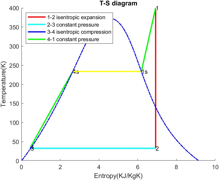
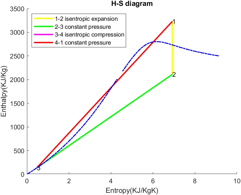
Rankine cycle simulator
1-2 isentropic expansion in the turbine
2-3 constant pressure heat rejection by condenser
3-4 isentropic compression in the pump
4-1 constant pressure heat addition by boiler
temperature at turbine inlet(in degree celcius): 400
pressure at turbine inlet(in bar): 30
pressure at turbine outlet(in bar): 0.05

at state point 1:
p1 is: 30.000000 Bar
t1 is : 400.000000 deg celcius
h1 is: 3231.571027 KJ/Kg
s1 is: 6.923259 KJ/KgK

at state point 2:
p2 is: 0.050000 Bar
t2 is : 32.875490 deg celcius
h2 is: 2110.708212 KJ/Kg
s2 is: 6.923259 KJ/KgK
x2 is: 0.814256

at state point 3:
p3 is: 0.050000 Bar
t3 is : 32.875490 deg celcius
h3 is: 137.765119 KJ/Kg
s3 is: 0.476254 KJ/KgK

at state point 4:
p4 is: 30.000000 Bar
t4 is : 36.834000 deg celcius
h4 is: 140.762226 KJ/Kg
s4 is: 0.476254 KJ/KgK

wt is: 1120.862815 KJ/Kg
wp is: 278.527345 KJ/Kg
wnet is: 842.335471 KJ/Kg
Ntherm is: 27.252914 percent
s.s.c is: 3.211811 Kg/Kwh