Week 4.1 - Genetic Algorithm
objective:
to develop a code to optimize the stalagmite function and to find the global maxima of it.
genetic algorithm:
it is derived with the help of chales darwin's theory of natural selection where to fit individuals are crossed to produce an offspring that can tackle the challenges around better than the previous generation.
the way it works is it moves on from one process to another, they are
1.initialisation
2.selection of parents and crossover
3.mutation of offspring
4.merge main and offspring
if all goes well terminate the function for the desired output received.
that is from two individuals another set of individuals are produced by crossing and the new born individuals are checked for the mutation, that makes them different from the parent individuals and are monitored inorder to attain a definite required sustainability of the changing environment.
stalagmite function for the code:
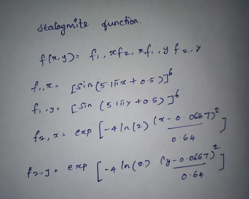
code for the above function:
function[f] = stalagmite(input_value)
%intialising x and y input values
x = input_value(1);
y = input_value(2);
%tx1 for f1x and ty1 for f1y
tx1 = (sin(5.1*pi*x + 0.5))^6;
ty1 = (sin(5.1*pi*y + 0.5))^6;
%tx2 for f2x and ty2 for f2y
tx2 = exp(-4*log(2)*((x-0.0667)^2/0.64));
ty2 = exp(-4*log(2)*((y-0.0667)^2/0.64));
f = tx1*ty1*tx2*ty2;
end
the code is provided with the above given values.
genetic algorithm code:
clear all
close all
clc
%genetic algorithm search space
x = linspace(0,0.6,150);
y = linspace(0,0.6,150);
%2dimensional mesh
[xx,yy] = meshgrid(x,y);
%evaluating stalagmite function
for i = 1:length(xx)
    for j = 1:length(yy)
        input_value(1)=xx(i,j);
        input_value(2)=yy(i,j);
        f(i,j) = stalagmite_func(input_value);
    end
end
%creating a stalagmite
surfc(xx,yy,f)
xlabel('x value')
ylabel('y value')
%to hide grid
%shading to remove grid
shading interp

[inputs,fval] = ga(@stalagmite,2)
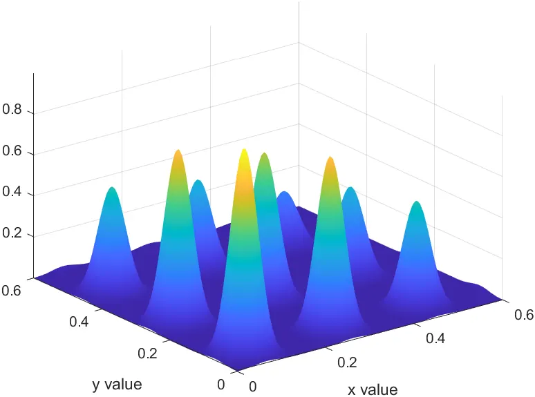
the above function defines the basic genetic algorithm code
image for the above genetic algorithm:
the ga syntax are as follows:
x = ga(fun,nvars)x, to the objective function, fun. nvars is the dimension (number of design variables) of fun.x = ga(fun,nvars,A,b)x to fun, subject to the linear inequalities A*x ≤ b. ga evaluates the matrix product A*x as if x is transposed (A*x').
x = ga(fun, nvars, A, b, Aeq, beq)
x = ga(fun,nvars,A,b,Aeq,beq)x to fun, subject to the linear equalities Aeq*x = beq and A*x ≤ b. (Set A=[] and b=[] if no linear inequalities exist.) ga evaluates the matrix product Aeq*x as if x is transposed (Aeq*x').
x = ga(fun, nvars, A, b, Aeq, beq, lb, ub)
x = ga(fun,nvars,A,b,Aeq,beq,lb,ub)x, so that a solution is found in the range lb ≤ x ≤ ub. (Set Aeq=[] and beq=[] if no linear equalities exist.)
x = ga(fun, nvars, A, b, Aeq, beq, lb, ub, nonlcon)
x = ga(fun,nvars,A,b,Aeq,beq,lb,ub,nonlcon)nonlcon. The function nonlcon accepts x and returns vectors C and Ceq, representing the nonlinear inequalities and equalities respectively. ga minimizes the fun such that C(x) ≤ 0 and Ceq(x) = 0. (Set lb=[] and ub=[] if no bounds exist.)
x = ga(fun, nvars, A, b, Aeq, beq, lb, ub, nonlcon, options)
x = ga(fun,nvars,A,b,Aeq,beq,lb,ub,nonlcon,options)options.
x = ga(fun, nvars, A, b, Aeq, beq, lb, ub,nonlcon, intcon)
x = ga(fun,nvars,A,b,Aeq,beq,lb,ub,nonlcon,intcon)x = ga(fun,nvars,A,b,Aeq,beq,lb,ub,nonlcon,intcon,options)intcon take integer values.
x = ga(fun, nvars, A, b, Aeq, beq, lb, ub, nonlcon, intcon, options)
x = ga(problem)problem
[, for any previous input arguments, also returns x,fval] = ga(___)fval, the value of the fitness function at x.
[x,fval,exitflag,output] = ga(___)
[ also returns x,fval,exitflag,output] = ga(___)exitflag, an integer identifying the reason the algorithm terminated, and output, a structure that contains output from each generation and other information about the performance of the algorithm.
[x,fval,exitflag,output,population,scores] = ga(___)
[ also returns a matrix x,fval,exitflag,output,population,scores] = ga(___)population, whose rows are the final population, and a vector scores, the scores of the final population.
..............................................................................................................................................................................................................................................................................................................................................................
study code 1:
clear all
close all
clc
%search area
x = linspace(0,0.6,150);
y = linspace(0,0.6,150);
%no of times ga runs
num_time = 50;
%creating 2d
[xx,yy] = meshgrid(x,y);
%stalagmite function
for i = 1:length(xx)
    for j = 1:length(yy)
        input_value(1)=xx(i,j);
        input_value(2)=yy(i,j);
        f(i,j) = stalagmite_func(input_value);
    end
end
%study 1 - statistical behaviour
%time count
tic
for i = 1:num_time
    [inputs,fopt(i)] = ga(@stalagmite,2);
    xopt(i) = inputs(1);
    yopt(i) = inputs(2);
end
study1_time = toc

%plot
figure(1)
subplot(2,1,1)
hold on
%creating stalagmite
surfc(x,y,-f)
xlabel('x value')
ylabel('y value')
%removing grid
shading interp
%using plot3 command
plot3(xopy,yopt,-fopt,'marker','o','markersize',5,'markerfacecolor','r')
title('unbound inputs')
subplot(2,1,2)
plot(-fopt)
xlabel('iterations')
ylabel('function minimum')
explanation for 1:
we start with clear all,close all and clc as always.
search area for the ga is bounded as x and y. from 0 to 0.6 into 150 divisions.
x = linspace(0,0.6,150);
y = linspace(0,0.6,150);
time for ga to run:
number of checktime is stated as 50
followed by all we create a 2 dimensional view from x and y
[xx,yy] = meshgrid(x,y);
we create a stalagmite funnction code.we increment i value and for all i we increment j. we then assign the input values and then calling stalagmite function for value of f
%stalagmite function
for i = 1:length(xx)
for j = 1:length(yy)
input_value(1)=xx(i,j);
input_value(2)=yy(i,j);
f(i,j) = stalagmite_func(input_value);
end
end
followed by we create a code for the time count and the ga.
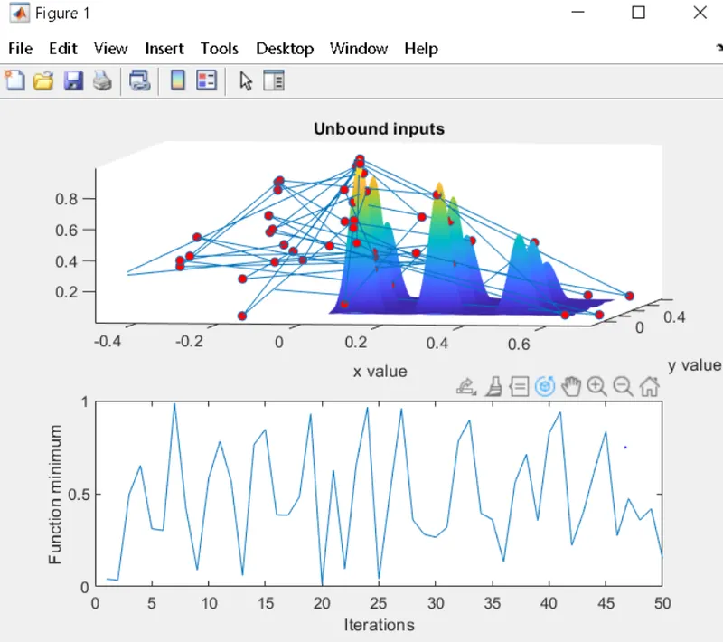
followed by all we create a plot, figure 1 which contain the main plot and subplot for better understanding
the grid function is made off with use of shading interp.
plot:
study 2:
code:
clear all
close all
clc
%search area
x = linspace(0,0.6,150);
y = linspace(0,0.6,150);
%no of times ga runs
num_time = 50;
%creating 2d
[xx,yy] = meshgrid(x,y);
%stalagmite function
for i = 1:length(xx)
    for j = 1:length(yy)
        input_value(1)=xx(i,j);
        input_value(2)=yy(i,j);
        f(i,j) = stalagmite_func(input_value);
    end
end
%study 2 - statistical behaviour
%time count
tic
for i = 1:num_time
    [inputs,fopt(i)] = ga(@stalagmite,2,[],[],[],[],[0:0],[0.5:0.5]);
    xopt(i) = inputs(1);
    yopt(i) = inputs(2);
end
study2_time = toc

%plot
figure(2)
subplot(2,1,1)
hold on
%creating stalagmite
surfc(x,y,-f)
xlabel('x value')
ylabel('y value')
%removing grid
shading interp
%using plot3 command
plot3(xopy,yopt,-fopt,'marker','o','markersize',5,'markerfacecolor','r')
title('Bound inputs')
subplot(2,1,2)
plot(-fopt)
xlabel('iterations')
ylabel('function maximum')
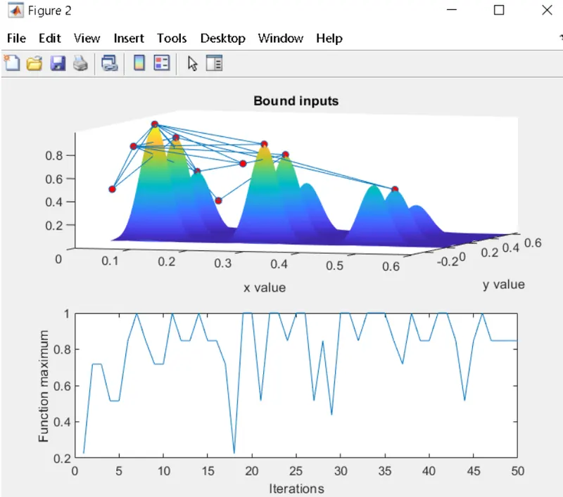
explanation is similar to 1 with few changes in second code inside and the names.
plot:
study 3:
code:
clear all
close all
clc
%search area
x = linspace(0,0.6,150);
y = linspace(0,0.6,150);
%no of times ga runs
num_time = 50;
%creating 2d
[xx,yy] = meshgrid(x,y);
%stalagmite function
for i = 1:length(xx)
    for j = 1:length(yy)
        input_value(1)=xx(i,j);
        input_value(2)=yy(i,j);
        f(i,j) = stalagmite_func(input_value);
    end
end
options = optimoptions('ga')
options = optimoptions(options,'populationsize',360)
%study 3
%time count
tic
for i = 1:num_time
    [inputs,fopt(i)] = ga(@stalagmite,2,[],[],[],[],[0:0],[0.5:0.5],[],[],options);
    xopt(i) = inputs(1);
    yopt(i) = inputs(2);
end
study2_time = toc

%plot
figure(3)
subplot(2,1,1)
hold on
%creating stalagmite
surfc(x,y,-f)
xlabel('x value')
ylabel('y value')
%removing grid
shading interp
%using plot3 command
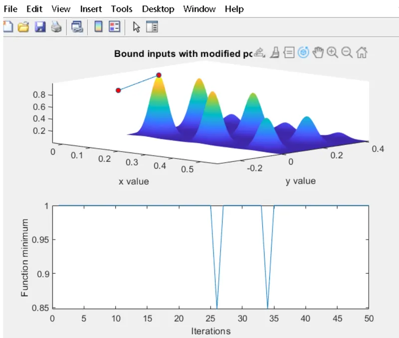
plot3(xopy,yopt,-fopt,'marker','o','markersize',5,'markerfacecolor','r')
title('Bond inputs with modified population size')
subplot(2,1,2)
plot(-fopt)
xlabel('iterations')
ylabel('function minimum')
explanation is similar as we are trying to achieve a global max with few change in names and the ga function.
plot:
error:
didnt come across much errors, only few like the name mismatch in the function code and main code
conclusion:
found the resourses from different youtube videos and matlab website.
1.https://in.mathworks.com/help/gads/how-the-genetic-algorithm-works.html
time:
time for 1 = 2.54 sec
time for 2 = 3.44 sec
time for 3 = 21.58 sec
f value is converted to -f as the ga always gives the minimum value.