Week 5 - Curve fitting

OBJECTIVE:

• To fit a linear and cubic polynomial for a given data and to show whether the result is good or bad.

THEORY:

Curve fitting is a process of determining a best possible curve for a given data . This method is useful for extrapolation or interpolatio of data . In simple words, curve fitting process can be used to find a data outside the given range.

There are various type of curve fitting process and the use of these process depends on the type of data given. They are

• Linear curve fitting - fitting of first order polynomial to a data
• Cubic curve fitting-fitting of third order polynomial to a data
• Highrt order curve fitting - fitting of higher order polynomial to a data
• Curve fitting using a splitwie polynomial method-using different /same order polynomial for the different divisions (parts) of given data range.

PROBLEM STATEMENT:

1. To explain what does popt and pcov mean
2. To explain what does np.array(temperature) do
3. To explain what does the * in *popt mean
4. To write the code to fit a linear and cubic polynomial for the Cp data and find whether the results are good or bad.
5. To explain the needs to be done in order to make the curve fit perfect
6. To show empirically , how well the curve has been fit.

SOLUTION :

1. popt and pcov:

'popt' and 'pcov' are the output arguments of the python's inbuilt function 'curve_fit' imported from 'scipy' module.

1. popt- An array of optimal values for the parameters which minimizes the sum of squares of residuals.

   pcov-2d array which contains the estimated covariance of popt. The diagonals provide the variance of the parameter estimate.

2. np.array(temperature): The command 'np.array(temperature)' is used for accessing the individual elements of the temperature array with the help of numpy module. Numpy module is imported as 'np' and used to perform mathematical operations like addition , substraction, multiplication,division,etc. on each element of the array or between the array.
3. '*' in popt :

   The star i.e. '*' in 'popt' unpacks the 'popt' array so that the optimized coefficients (parameters) values can be accessed from the array 'popt'. In others, '*' (* means all) aids in referring to all the values stored in the array 'popt'.

4. Code to fit a linear and cubic polynomial for the Cp data:

#Code to perform curve fitting using linear and cubic polynomial

#importing the requied modules
import math
import matplotlib.pyplot as plt
import numpy as np
from scipy.optimize import curve_fit


#Define a function to read the data file containing temperature and cp values
def read_file():
	temperature=[]
	cp=[]
	# for loop for reading the data file line by line and preparing the data
	for line in open('data','r'):
		values=line.split(',')
		temperature.append(float(values[0]))
		cp.append(float(values[1]))
	return[temperature,cp]

#Calling the function read_file to get temperature and cp values
temperature,cp=read_file()

#Performing curve fitting using Linear Polynomial
#Function to define the linear polynomial for curve fitting
'''
Linear polynomial 
cp = a*T+b

Cubic polynomial
cp = at^3 +bt^2 +ct +d
'''

#function for linear polynomial
def linear(t,a,b,c,d):
	return(a*t + b)
#function for cubic polynomial
def cubic(t,a,b,c,d):
	return(a*pow(t,3)+b*pow(t,2)+c*t+d)


#for linear equation
popt1,pcov1=curve_fit(linear,temperature,cp)
fit_cp1=linear(np.array(temperature),*popt1)

#for cubic equation
popt,pcov = curve_fit(cubic,temperature,cp)
fit_cp=cubic(np.array(temperature),*popt)


#plotting for linear equation
plt.figure(1)
plt.plot(temperature,cp,color='blue',Linewidth=3)
plt.plot(temperature,fit_cp1,color='red',Linewidth=3)
plt.xlabel('Temperature[K]')
plt.ylabel('Cp')

#Plotting for cubic equation
plt.figure(2)
plt.plot(temperature,cp,color='blue',Linewidth=3)
plt.plot(temperature,fit_cp,color='red',Linewidth=3)
plt.xlabel('Temperature[k]')
plt.ylabel('Cp')
plt.show()

Procedure:

• The required modules are imported.
• Curve_fit function is imported from the scipy module is used to determine the true nature of the given curve
• The read_file() function is defined to read the data from the file which contains the specific heat values for the given temperatures which are seperated by comma . So, inside that function the split command is used to split both the values and store them in the two different array.
• Next the read function was called and then the values are stored in temperature and cp
• popt,pocv=curve_fit(linear,temperature,cp) . This code is given to fetch theco-efficient required for the linear polynomial expression , the curve fit function calculates thevalue for the co-efficient and stores them in the 'popt' and their covarience values are stored in the 'pcov'
• fit_cp1= linear(np.array(temperature).*popt). This code is given to call the linear function by passing the values of the temperature list as numpy array with *popt which has the values of co-efficient for the other parameters in the function.
• The same steps are repeated for the cubic polynomial.
• Then the values stored in the fit_cp1(cp values for linear function) and fit_cp2(cp values for cubic function ) were plotted along with the temperature values.

result:

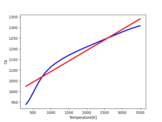
Linear polynomial ,

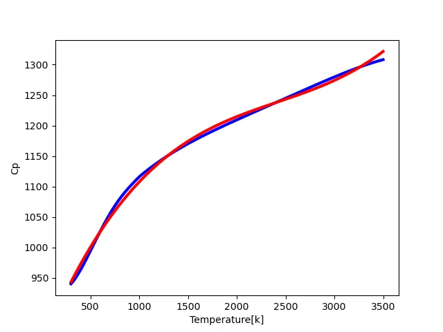
Cubic polynomial,

observation:

It is clear from the above graph that the curve fits better when the degree of the polynomial increases. It is observered that tha deviation of the curve fit with actual data is more for linear equation and gradually the deviation decreases with the increase in the order of the polynomial.

V. Needs to be done in order to make the curve fit perfect:

A curve fit can almost never be perfect because experimental data will always vary from a perfect equation .However the fit can be made as close as possible by trying different order equations, extrapolation ,dividing the data and curve fitting them seperately or on very rare case finding an equation which fits the data perfectly.

VI . Empirically shown:

As empirically we can conclude that the order or the degree of equation increases, we get less deviation ,so that best curve fit can be obtained.