Pipe flow simulation

AIM:

To run a pipe flow simulation with an inlet Reynolds number of 100,1000 and 10,000.

For each of these cases do the following

1.line probes at 95%, 90% and 85% of the pipe length.

2. To compare the normalized velocity profile at each of these locations

3. To normalize the velocity profile by the inlet velocity.

Theory:

The fluids can be classified into different types based on the variation of the fluid characteristics like velocity, density etc. Depending on the type of flow, the analysis method varies in fluid mechanics.

The different types of fluid flow are:

1. Steady and Unsteady Flow
2. Uniform and Non-Uniform Flow
3. Laminar and Turbulent Flow
4. Compressible and Incompressible Flow
5. Rotational and Irrotational Flow
6. One, Two and Three -dimensional Flow

Laminar and Turbulent flow in a pipe flow is characterised based on Reynold number.

Reynold's number:

The Reynolds number is the ratio of inertial forces to viscous forces within a fluid which is subjected to relative internal movement due to different fluid velocities, in what is known as a boundary layer in the case of a bounding surface such as the interior of a pipe

The Reynolds number is defined as

Laminar flow:

Laminar flow is defined as a type of flow in which the fluid particles move along a well-defined streamline or paths, such that all the streamlines are straight and parallel to each other.

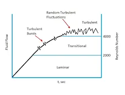
The flow is laminar when the Reynolds number is less than 2000.

Turbulent flow:

Turbulent flow is a type of flow in which the fluid particles move in a zig-zag manner. The movement in zig-zag manner results in high turbulence .

The flow is turbulent when the Reynolds number is greater than 4000.

Transition state:

The flow is in transition state when reynolds number is between 2000 and 4000.

Flow simulation:

Flow Simulation enables users to simulate a wide variety of liquids and gases for different engineering scenarios. A few common applications are flow through pipes, flow through manifolds, heat exchangers, electronics cooling and aerodynamics.

Calculation:-

We have three case of Reynold's number using which we will find the velocity and length of the pipe. In this case let's take,

External diameter = 40mm =0.04 m Internal diameter = 38mm =0.38 m Pipe Thickness = 2mm =0.002 m Pipe length = 1000mm =1 m density of water = 1000kg/m^3 viscosity of water =0.001 pa s

Calcutaion of velocity:

Re =(ρVL)/μ

CASE 1 (Re = 100)	100= (1000*V*0.038)/0.001	V=0.00263157 m/s
CASE 2 (Re= 1000)	1000=(1000*V*0.038)/0.001	V=0.0263157 m/s
CASE 3 (Re=10000)	10000=(1000*V*0.038)/0.001	V=0.263157 m/s

Procedure:

STEP 1:

Open a new part workpage and set the plane . Set the unit in mks

STEP 2:

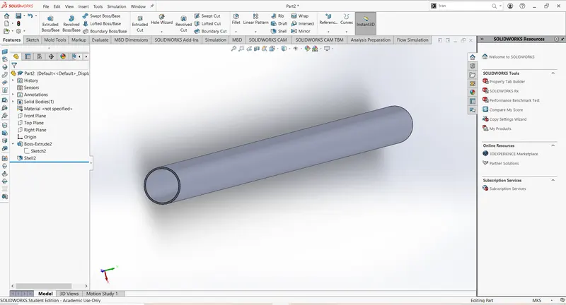
Design a pipe with a given measurements ( D=0.04 m , d= 0.038m , L =1m). Draw a circle of diameter 0.04m and extrude it to a length of 1m . Using shell option make it hollow with the thickness 0.002m .

STEP 3:

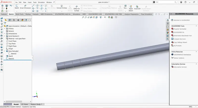
Creating line probe

CASE 1	95%	0.95m
CASE 2	90%	0.9m
CASE 3	85%	0.85m

STEP 4 :

Open flow simulation in solidworks. Seal the pipe using the option create lids. And now we have to define the project in flow simulation.To achieve that we are using wizard option . The following table is being defined using wizard option,

Project name	Pipe simulation
Analysis type	Internal
Type of fluid	Liquid(water)
Type of flow	Laminar and turbulent
Thermal condition	Adiabatic wall
Roughness	0 micrometer

STEP 5:

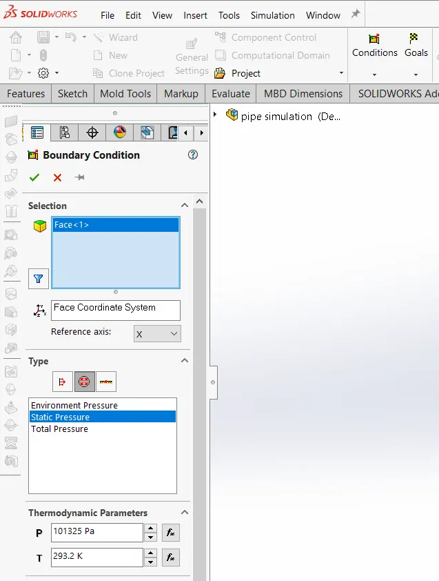
To define the boundary conditions, right click on boundary conditions and the click on insert boundary conditions

At outlet,

static pressure 101325 pa , 293.2k

At inlet ,

inlet velocity as follows,

Case 1	V=0.00263157 m/s
Case 2	V=0.0263157 m/s
Case 3	V=0.263157 m/s

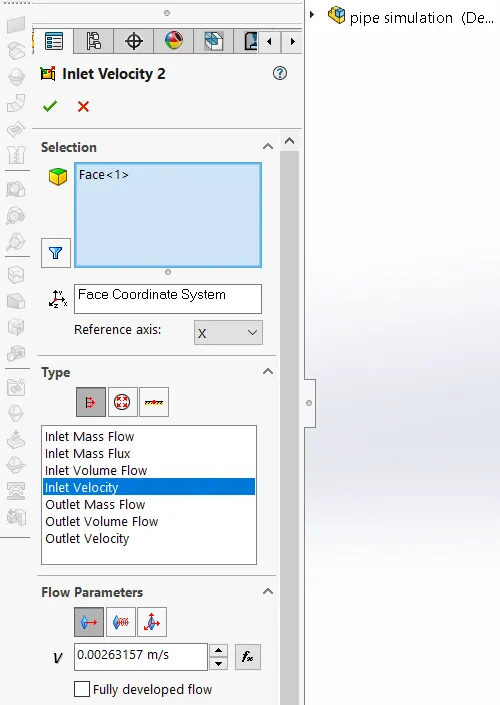
insert another boundary condition for the wall (real wall)

STEP 6:

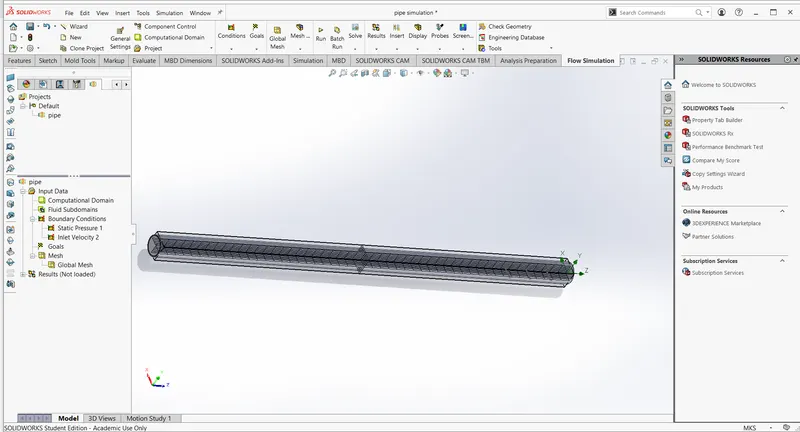
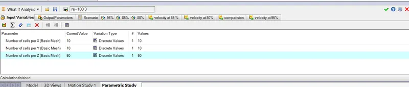
Now we have to set the mesh manually Nx =10 ; Ny = 10 ; Nz = 50

STEP 7:

To get the result we have to plot XY-plots for velocities at each probe location (i.e 95%,85%,80% of the pipe length)

STEP 8:

Create cut plot near each probe location making pipe transparent.

STEP 9:-

Run the simulation.

SIMULATION AND ANALYSIS:

STEP 1:

Set the input variables

STEP 2 :

Set the output parameters

STEP 3 :

Set the senario . In this I have made 3 column each design point increases with a factor of 1,2,4 respectively.From this we get 3 different sized mesh .

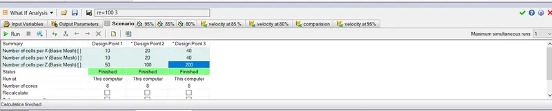
In this we have taken three design points , starting from low number of mesh to high number of mesh.

SIMULATION RESULT:

In simualtion result we consider the better result . We get the better result when our mesh number is higher.

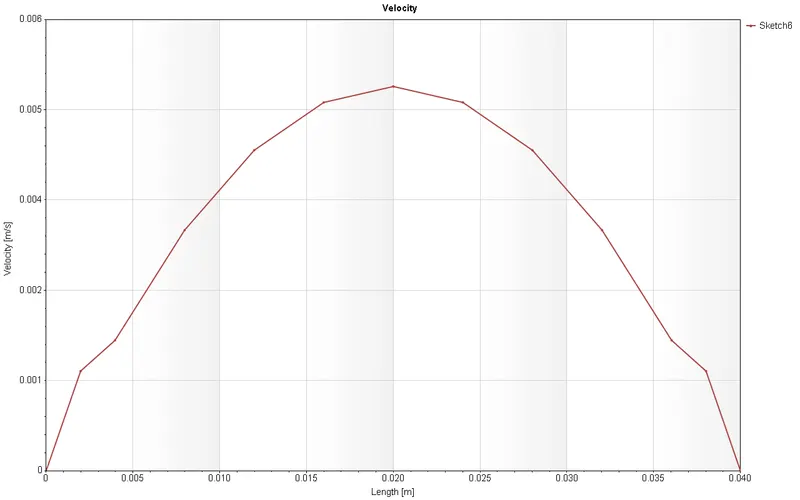
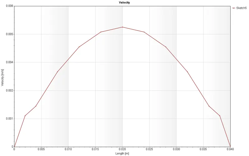
CASE 1: ( Re=100)

AT 95% OF THE LENGHT OF THE PIPE

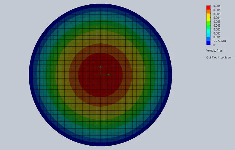
velocity graph

AT 85% OF THE LENGHT OF THE PIPE

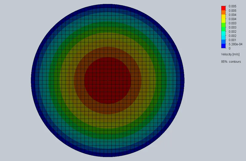
velocity graph

AT 80% OF THE LENGHT OF THE PIPE

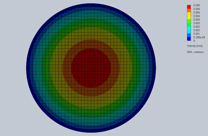
velocity graph,

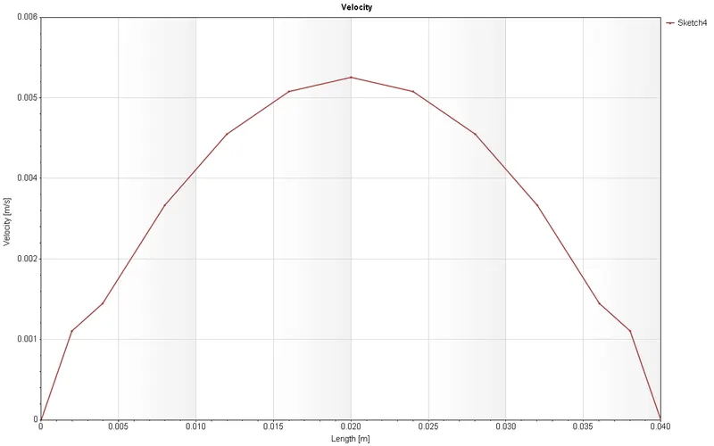
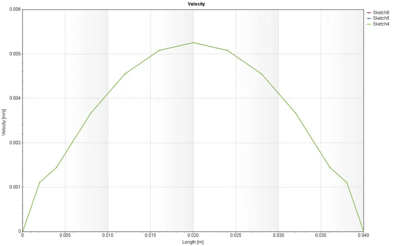
comparison of velocity graph when Re=100 at 95% , 85% , 80% of the pipe length

CASE 2: ( Re=1000)

AT 95% OF THE LENGHT OF THE PIPE

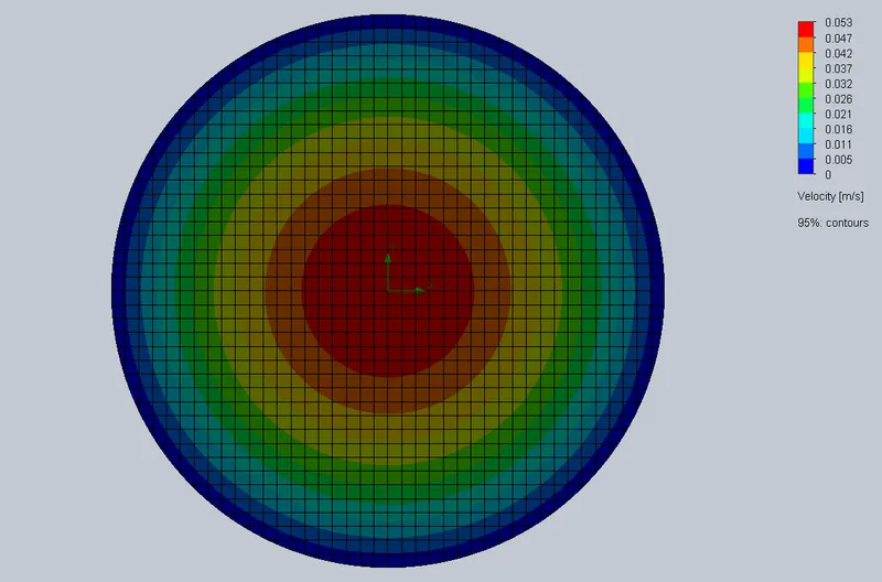
velocity graph,

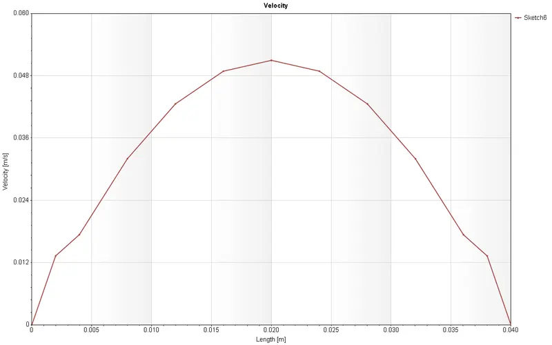
AT 85% OF THE LENGHT OF THE PIPE

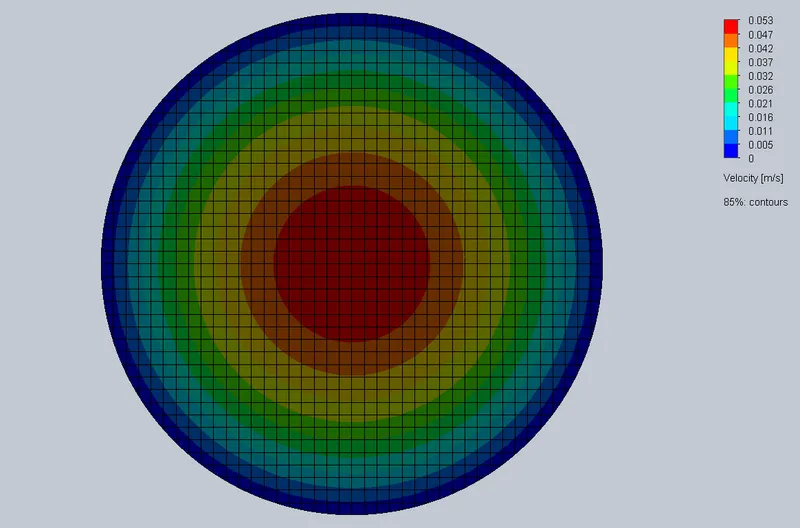
velocity graph,

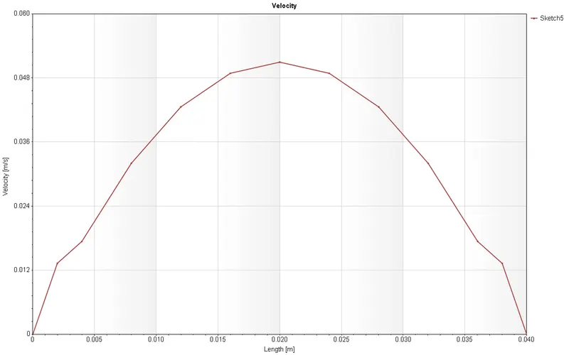
AT 80% OF THE LENGHT OF THE PIPE

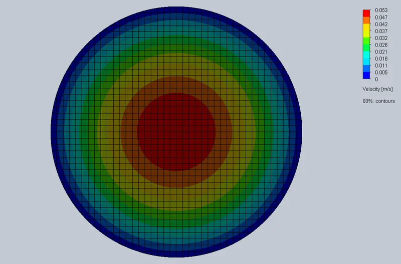
velocity graph,

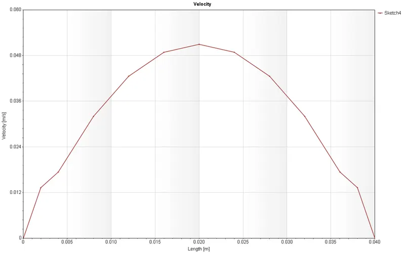
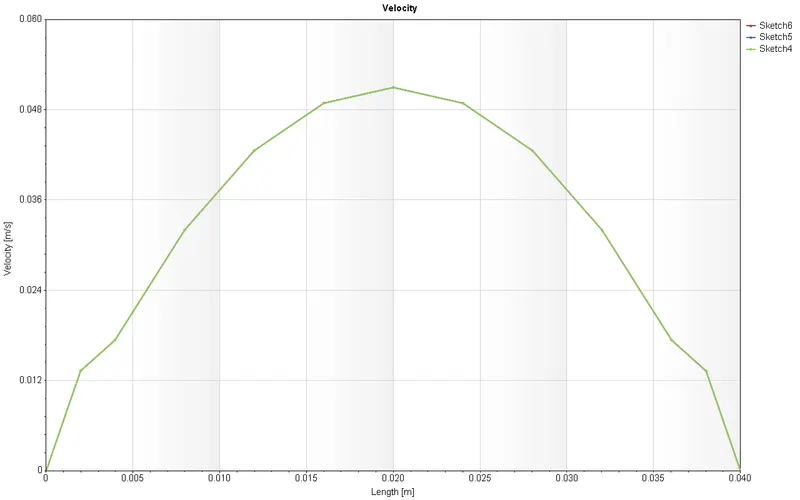
comparison of velocity graph when Re=1000 at 95% , 85% , 80% of the pipe length

CASE 3: ( Re=10000)

AT 95% OF THE LENGHT OF THE PIPE

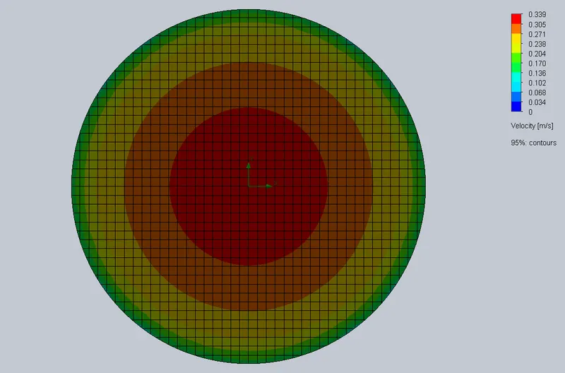
velocity graph,

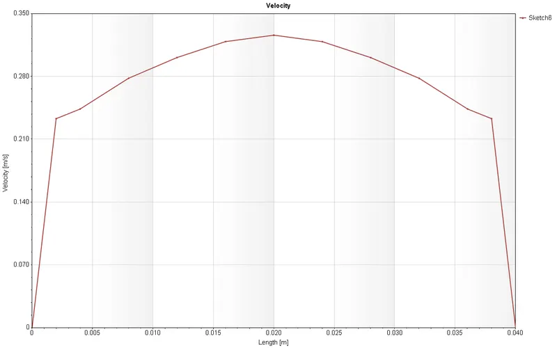
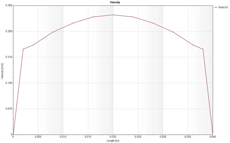
AT 85% OF THE LENGHT OF THE PIPE

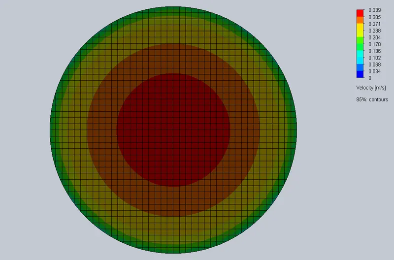
velocity graph,

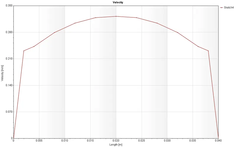
AT 80% OF THE LENGHT OF THE PIPE

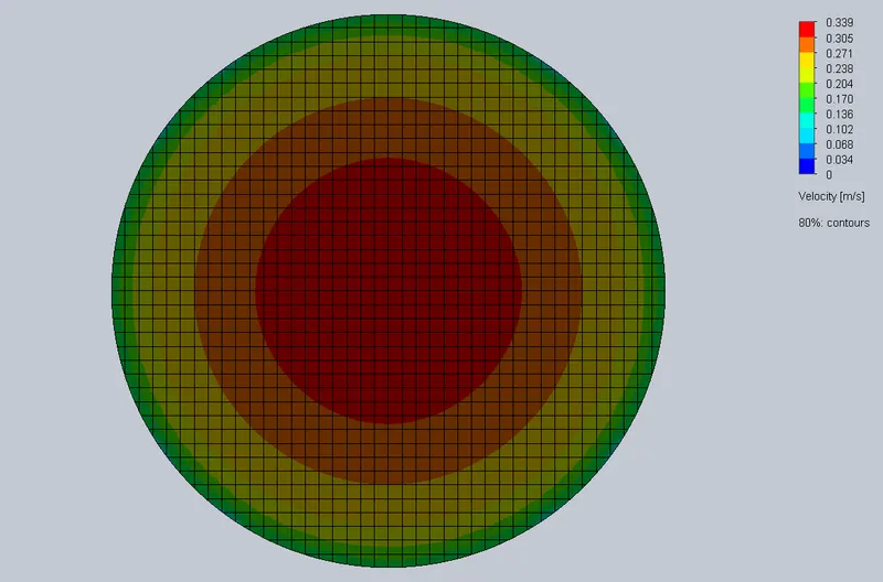
velocity graph,

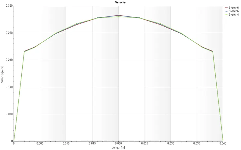
comparison of velocity graph when Re=10000 at 95% , 85% , 80% of the pipe length

CONCLUSION:

• As the size of mesh increases the accuracy also increases
• In case 1 and 2 the velocity profilr is parabolic in nature.
• As Reynold's number is less than 2000 (i.e Re100 &1000) in case 1 and 2 it is laminar flow.
• In case 3 the velocity profile is not parabolic it is logarithemic.
• As the Reynold's number is more than 4000 (i.e 10000)in case 3 it is turbulent flow.
• The probe used in our study indicates that the velocity changes unlit the flow is fully developed after that the velocity in the pipe is constant. The length about which the flow is getting fully developed is based on Poisulle's Theorem.
• As the Reynolds number increases the velocity in the pipe till fully developed flow is increases. also, the velocity profile change indicate that the change in flow is from Laminar to turbulent .Hence, we can conclude that the type of flow depends upon the Reynolds number.