Week 5 - Curve fitting

Aim: To perform curve fitting using Python code.

Theory:

Curve fitting Is the process of constructing a curve, or mathematical function, that represents a series of data point closely. From curve fitting one can established a functional relationship between observed data points and parameter values. Etc. By doing curve fitting variation of a data can be predicted in a future. Accuracy of curve fit depends upon degree of polynomial. Higher the degree of polynomial, higher the accuracy of a curve fitting.

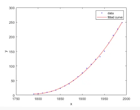
Figure: Curve fitting

Perfect fit and best fit are the important terms related to curve fitting.

Curve fitting is perfect if the distance between the data points and curve got after curve fitting is zero. Means curve passes exactly through points.

Curve fitting is best if the distance between the fitted curve and data points is minimum.

Python code

# Program for curve fitting 
import math
import numpy as np
import matplotlib .pyplot as plt
from scipy.optimize import curve_fit

#curve fit function(linear) 

def func(t,a,b):
	return a*t + b

#reading the thermodynamic data file 

def read_file():
	temperature = [] 
	cp = []
	for line in open('data','r'):
		values = line.split(',')
		temperature.append(float(values[0]))
		cp.append(float(values[1]))

	return [temperature,cp]

#Main program
temperature, cp = read_file()
popt,pcov = curve_fit(func,temperature,cp) 
fit_cp = func(np.array (temperature), *popt) 
print(popt)

# To plot results for linear curve fit
plt.plot(temperature, cp,color='blue',linewidth=3) 
plt.plot(temperature, fit_cp,color='red',linewidth=3) 
plt.legend(['Actual data','Linear Curve fit'])
plt.xlabel('temperature [K]')
plt.ylabel('specific heat at constant pressure Cp')
plt.savefig('plot 1') 
plt.grid()
plt.show()

#cubic fit function(cubic polynomial) 

def func(t,a,b,c,d):
	return a*pow(t,3)+b*pow (t,2)+ c*t+d

#reading the data file provided 
def read_file ():
	temperature = []
	cp = []
	for line in open( 'data' ,'r'): 
		values = line.split (',')
		temperature .append(float(values[0]))
		cp.append(float(values[1]))

	return [temperature, cp]


#Main program
temperature, cp = read_file ()
popt, pcov = curve_fit(func, temperature, cp)
fit_cp = func(np.array(temperature), *popt) 
print(popt)

# To plot results for Cubic curve fit
plt.plot(temperature, cp,color='blue',linewidth=3) 
plt.plot(temperature, fit_cp,color='red',linewidth=3) 
plt.legend( ['Actual data','Cubic curve fit']) 
plt.xlabel('temperature [K]')
plt.ylabel('specific heat at constant pressure Cp')
plt.savefig('plot2')
plt.grid()
plt.show ()

• In program popt is used to find out values of constants of curve fit equation like a,b,c etc.
• pcov contains convarient matrix, which indicates uncertees and corelation between parameters. This is mostly applicable when data has uncertainties.
• In the code *popt refers to the value of a coeficients calculated by popt function
• In the code np.array is used to store different values of temperature.

Results and conclusion

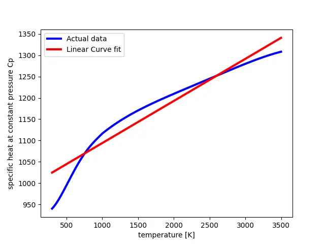
Figure: Linear curve fit

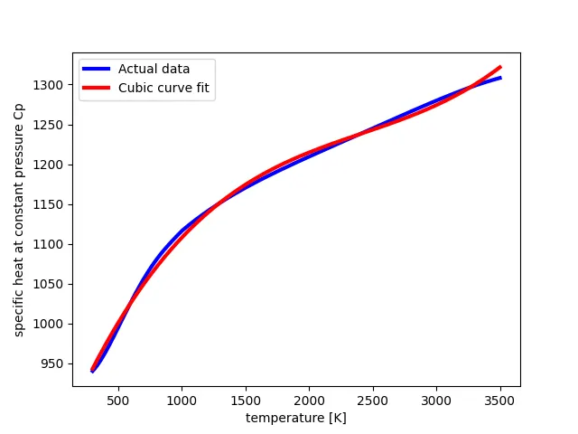
Figure: Cubic curve fit

• From above figures it is seen that, linear curve fit does not represent the accurate representation of the data as curve for linear data is not matching with actual data'
• Cubic curve fit curve is matching with actual data curve. It means given data can be best represented by cubic curve fit rather than actual curve fit.
• So in general to improve qulaity of curve fit, one needs to use higher degree polynomial