Week 3 - Solving second order ODEs

OBJECTIVES

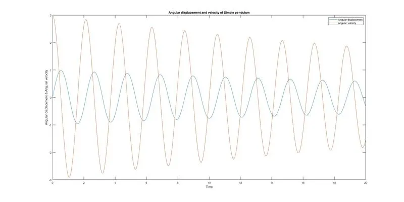
• Write a MATLAB program to solve the second order ODE which define motion of a simple pendulum and plot the graph of Angular displacement and velocity
• Create an animation showing motion of simple pendulum.

THEORY

• Pendulum

A pendulum is a weight hung from a stationary point in a way that allows it to swing freely back and forth. A pendulum is consist of a string,mass and a fixed point. A simple pendulum is one where the pendulum bob is treated as a point mass, and the string from which it hangs is of negligible mass.

The ODE that we want to solve is given below, This ODE represents the equation of motion of a simple pendulum with damping.

`(d^2theta)/(dt^2)+(b/m)(d theta)/(dt)+(g/l)sintheta=0`

Where,

b = Damping coefficient

m = Mass of the bob in kg

g = Acceleration due to gravity in `m/s^2`

l = length of the pendulum in m

• Damping

Damping is an influence within or upon an oscillatory system that has the effect of reducing or preventing its oscillation. In physical systems, damping is produced by processes that dissipate the energy stored in the oscillation.

ODE SOLVING PROCEDURE

Since it is a 2nd order ODE, inorder to solve that, we have to break them into 2 first order ODEs.

The equation of motion of simple pendulum is,

`(d^2theta)/(dt^2)+(b/m)(d theta)/(dt)+(g/l)sintheta=0`

Assume, `theta=theta_1`

So `(d theta)/dt=(d theta_1)/dt=theta_2`

`(d theta_1)/dt=theta_2`.............................eqn(1)

So 2nd order ODE becomes,

`(d^2theta_1)/(dt^2)+(b/m)(d theta_1)/(dt)+(g/l)sintheta_1=0`

`=>d/dt((d theta_1)/dt)+(b/m)theta_2+(g/l)sintheta_1=0`

Finally we get,

`(d theta_2)/(dt)=-(b/m)theta_2-(g/l)sintheta_1`.............................eqn(2)

These two 1st order ODEs are going to put in program as solution vector,

`[[(d theta_1)/dt],[(d theta_2)/dt]]=[[theta_2],[-(b/m)theta_2-(g/l)sintheta_1]]`

After that we are going to integrate them using ode45 function inorder to solve the ODE.

MATLAB CODE

• Function Code

function [dtheta_dt]=ode_fun(theta,t,b,g,m,l)
    
    % Defining solution vector
    theta1 = theta(1);
    theta2 = theta(2);
    dtheta1_dt = theta2;
    dtheta2_dt = -(b/m)*theta2-(g/l)*sin(theta1);
    dtheta_dt = [dtheta1_dt;dtheta2_dt];

end

• Main Code

% MATLAB program to solve the Simple pendulum ODE

clear all
close all
clc

% Inputs

% Damping coefficient
b = 0.05;

% Acceleration due to gravity
g = 9.81;

% Length of the pendulum
m = 1;

% Mass of the ball
l = 1;

% Initial conition
theta_0 = [0,3];

% Time
t_span = linspace(0,20,300);

% Solving the ODE using ode45
[t,result] = ode45(@(t,theta)ode_fun(theta,t,b,g,m,l),t_span,theta_0);

% Plotting angular displacement-velocity graph
figure(1)
plot(t,result(:,1))
hold on
plot(t,result(:,2))
xlabel('Time')
ylabel('Angular displacement & Angular velocity')
legend('Angular displacement','Angular velocity')
title('Angular displacement and velocity of Simple pendulum')

% Angular displacement = Theta
theta = result(:,1);

% Counter variable
ct=1;

% for loop for animation
for i=1:length(theta)

    % fixed end
    x1 = 0;
    y1 = 2;
    
    % position of bob
    x2 = -l*sin(theta(i));
    y2 = -l*cos(theta(i));

    figure(2)
    plot([-1.5,1.5],[2,2],LineWidth=3.5)
    hold on
    plot([x1,x2],[y1,y2],LineWidth=2.5)
    plot(x2,y2,'o',MarkerSize=30,MarkerFaceColor='black',MarkerEdgeColor='black')
    hold off
    xlim([-2.5,2.5])
    ylim([-2.5,2.5])
    title('Simple Pendulum Animation')
    pause(0.03)

    M(ct) = getframe(gcf);
    ct=ct+1;
    
end

% Creating animation
movie(M)
videofile = VideoWriter('Pendulum Animation','Uncompressed AVI');
open(videofile)
writeVideo(videofile,M)
close(videofile)

CODE EXPLANATION

• function and end - Function command is used to define a function. Solution vector is defined inside the function. End keyword is used to terminate/exit from the function
• clear all - To clear all variables from the current workspace.
• close all - It closes all figures whose handles are visible.
• clc - clc clears all the text from the Command Window, resulting in a clear screen.
• linspace(0,20,300) - It generates 300 points between 0 and 20, which are equally spaced vectors.
• [t,result] = ode45(@(t,theta)ode_fun(theta,t,b,g,m,l),t_span,theta_0); - Using ode45 function inorder to solve the odes. Inside that we calling the previously defined function(Solution vector). And the next input is t_span which is the time interval to integrate the ode. Finally we defining the initial condition which is theta_0. Since we have two ODEs, we will have two initial conditions. 1 will give the Angular displacement and the 2nd one will give the angular velocity. These values are stored into result array. From this we can plot the angular diplacement-velocity diagram. And with the help of angular displacement values we can make the animation.
• plot - The plot function in Matlab is used to create a graphical representation of some data.
• hold on - hold on retains plots in the current axes so that new plots added to the axes do not delete existing plots.
• xlabel - It labels x-axis.
• ylabel - It labels y-axis.
• title - Add a title to a plot and return the text object.
• line 44 - Defining counter variable inorder to get the animation correctly.
• hold off - hold off sets the hold state to off so that new plots added to the axes clear existing plots and reset all axes properties.
• xlim - sets the x-axis limits for the current axes.
• ylim - sets the y-axis limits for the current axes.
• pause - It pauses execution for n seconds before continuing.
• x1,y1 - Defining the fixed point.
• x2,y2 - Defining the position of swinging end.
• plot([-1.5,1.5],[2,2],LineWidth=3.5) - Plotting fixed end.
• LineWidth - Line width is used to adjust the width of any object.
• plot([x1,x2],[y1,y2],LineWidth=2.5) - Plotting the string.
• MarkerSize - MarkerSize is used to control the overall size of markers.
• MarkerFaceColor - To set color in the marker.
• MarkerEdgeColor - To set color at the edge of the marker.
• M(ct) = getframe(gcf); - Creating M array to capture all movements.
• getframe - It captures the current axes as it appears on the screen as a movie frame.
• gcf - It returns the current figure handle.
• ct=ct+1; - Updating counter variable.
• movie(M) - movie(M) plays the movie frames in array M once.
• VideoWriter - Use a VideoWriter object to create a video file from an array.
• videofile = VideoWriter('Pendulum Animation','Uncompressed AVI'); - It additionally applies a set of properties tailored to a specific file format (such as 'MPEG-4' or 'Uncompressed AVI').
• open() - Open file for writing video data.
• writeVideo(videofile,M) - writes data from an array to the video file associated with M.
• close() - Close file after writing video data.

RESULT

• Angular displacement-Angular velocity diagram

• Pendulum Animation

https://drive.google.com/file/d/1N77zUdQV43z8_XbYJPvXNXonH1Y6fYI0/view?usp=sharing