Week 5 - Curve fitting

1. POPT:- is an array, Optimal values for the parameters so that the sum of squared residuals of f(xdata,*popt) - f(xdata, *popt) -ydata is minimized.In other words POPT is our coefficient, we have a,b,c,d are three unknowns so popt is going to be those values,Curve fit function is calculate them for us & popt is going to be an Output. PCOV:- is also an array, The estimated covariance of popt. The diagonals provide the variance of the parameter estimate.To compute one standard deviation errors on the parameters use perr = np.sqrt(np.diag(pcov)).
2. np.array(temperature) convert the temperature data in an array of shape 3200,shape can be obtained by using print(np.aaray(temperature).shape).
3. The star(*) in defination of the function wil accept the arguments supplied in the function that are not identified as a list.popt contains value for coefficient like a,b,c,d & *POPT helps us to refer those values.
4. AIM:- To write a code for linear and cubic polynomial

"""
code to fit a linear and cubic polynomial data for the cp data.

"""
import math
import matplotlib.pyplot as plt
import numpy as np

from scipy.optimize import curve_fit

#linear fit
def linear(t, a, b):
	return a*t + b  

# Reading thermo data file


temp = []
cp = []
	

for line in open('data', 'r'):
	values = line.split(',')
	temp.append(float(values[0]))
	cp.append(float(values[1]))
#print(temp)

popt,pcov=curve_fit(linear,temp,cp)
#print(popt)
plt.figure(1)
predicted_cp1=linear(np.array(temp),*popt)
plt.plot(temp,cp,color = "blue",linewidth=3)
plt.plot(temp,predicted_cp1,color="red",linewidth=3)
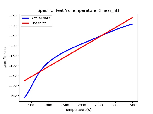
plt.title('Specific Heat Vs Temperature, (linear_fit)')
plt.legend(['Actual data', 'linear_fit'])
plt.xlabel('Temperature[K]')
plt.ylabel('Specific heat') 
plt.show()



# code to fit cubic polynomial

def poly_3(t,a,b,c,d):
	return a*pow(t,3)+b*pow(t,2)+c*t+d   

popt,pcov=curve_fit(poly_3,temp,cp)

predicted_cp3=poly_3(np.array(temp),*popt)
plt.figure(2)
plt.plot(temp,cp,color = "green",linewidth=3)
plt.plot(temp,predicted_cp3,color="red",linewidth=3)
plt.title('Specific Heat Vs Temperature, (Cubic_fit)')
plt.legend(['Actual data', 'Cubic_fit'])
plt.xlabel('Temperature[K]')
plt.ylabel('Specific heat') 
plt.show()

• Results Of Linear & Cubic Fit

1. Figure(1)

2

2.FIGURE(2)

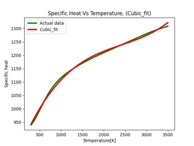
• Conclusion:- In linear fit data is not smoothly fixed & Actual data is scatterd but in Cubic fit the fitted curve overlaps the original curve except some regions.

5.In order to make perfect fit , we must consider error estimates, Perfect fit means, the curve should fit the original curve without showing any error in that particular degree of polynomial.Perfect fit can always be an best fit but best fit can not be a perfect fit.

Reference used:-

https://docs.scipy.org/doc/scipy/reference/generated/scipy.optimize.curve_fit.html