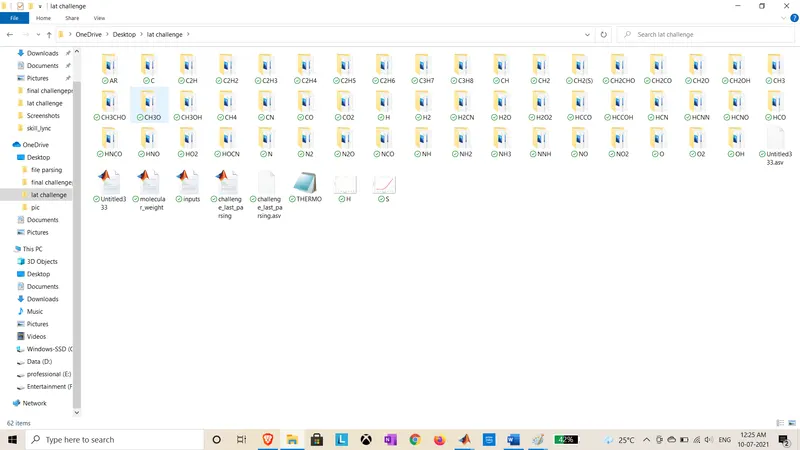
Project 1 - Parsing NASA thermodynamic data

AIM:-

1. To write a MATLAB code for parsing the NASA thermodynamic data file and to extract 14 coefficients thermodynamic properties like Cp,H,& S,for all species in the data file.
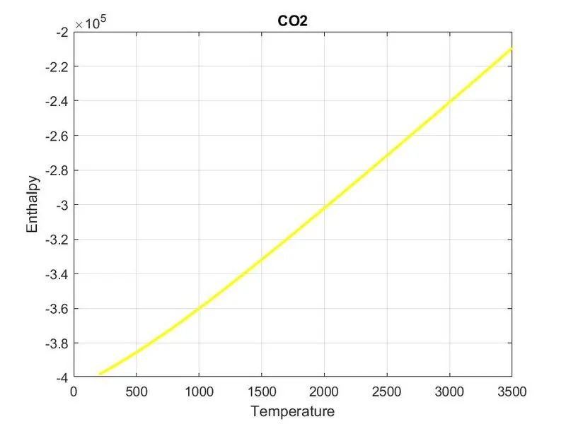
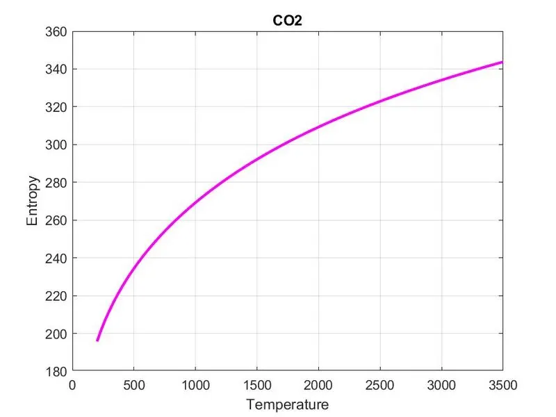
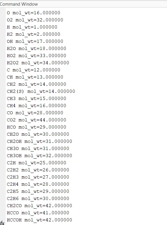
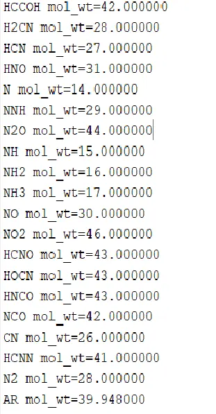
2. To find out the molecular mass of each species & finally to plot a graph of enthalpy,entropy & sp.heat with respect to Temprature.

THEORY:-

• FILE PARSING:- File parsing refers to how information can be read from text file or any type of file & how that information can be read in a program.The defination for parse is to split the file or other input into pieces or the data which can be easily stored or manipulated.
• Here we extract the data from the given thermodynamic data file & will calculate the Cp,H,& S for all species in data file.Also we are calculating the molecular wt. of each species.

FORMULA USED:-

• To calculate enthalpy,entropy and specific heat :

1. Cp/R = a1 + a2 T + a3 T^2 + a4 T^3 + a5 T^4
2. H/RT = a1 + a2 T/2 + a3 T^2/ 3 + a4 T^3/ 4+ a5 T^4 /5 + a6/T
3. S/R = a1 ln T + a2 T+ a3 T^2/2 + a4 T^3/3 + a5 T^4/ 4 + a7

The first 7 coefficients are high_Temperature coefficients and the second 7 coefficients are low_Temperature coefficients.

Also used the local temperature ranges which is unique for each individual species, not the Global temperature ranges.

EXPLAINATION:-

1. Clear all, close all and clc command is used to clear all workspace , clear the command window and closes the plot.
2. fopen command is used to open the THEMODAT FILE which is provided n 'r' is used to read thw data .
3. fgetl command is used to extract each line of the file . The first line is the Header information followed by Global temprature values. The next three lines are not required from program point of view.
4. The global temperature values obtained inprevious step is in the form of strings.In order to convert them into numbers we can used either str2num or str2double command is used.
5. onwards, we have 53 species name & their 14 coefficients.Using for loop,the name of the species & its coefficient are extracted.
6. the first fgetl command in loop gets us specious name.
7. the next three fget helps us extract the coefficient values.
8. The strfind command helps us to find the position of 'E' which is used as a reference for getting the coefficient values.
9. mkdir command is used to creates a folder for saving the plots that will be generated.
10. Range of temperature is assumed for calculating sp.heat, enthalpy & entropy values.
11. Then for loop determines these parameters for each temp values.
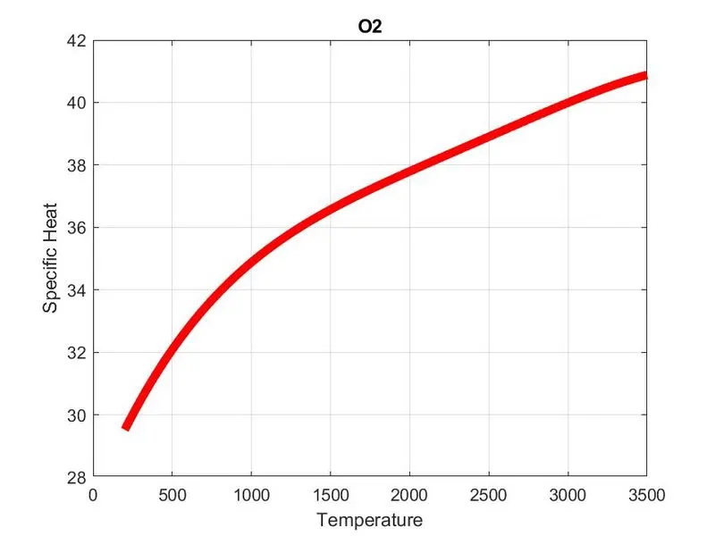
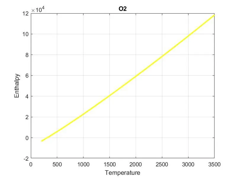
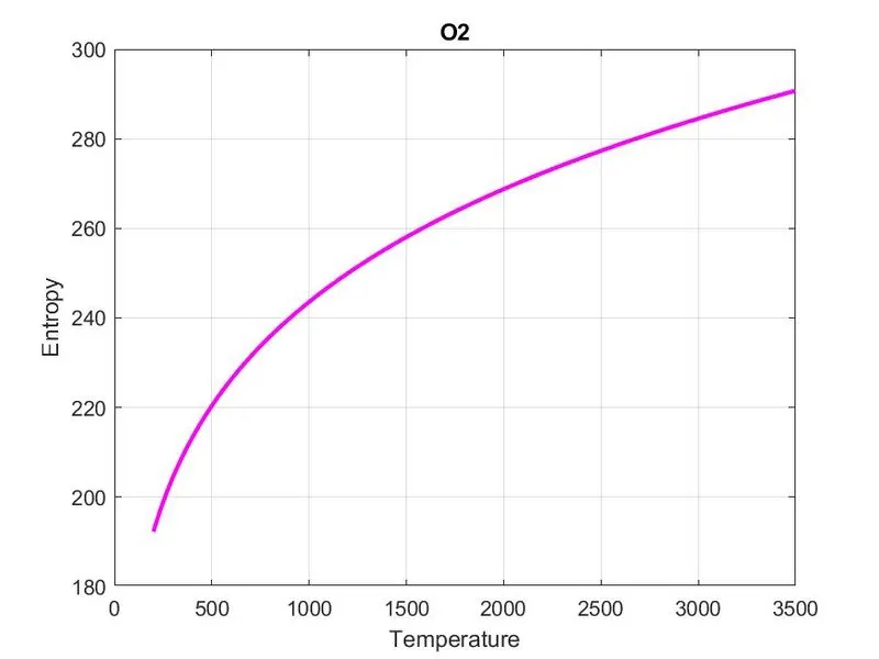
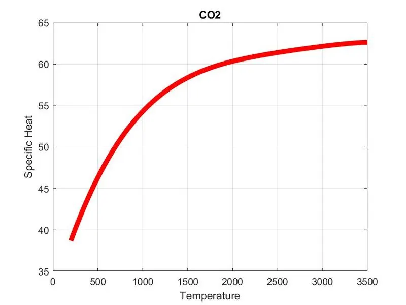
12. with the help of plot, all corresponding values of temprature is plotted.
13. the file directory is then changed.
14. save as command is ussed to saving those plots with names.
15. The directory is then switched back for molecular wt.
16. Then function is called to calculate molecular weight.

Main Program:-

clear all
close all
clc


%Extracting header_info
f1 = fopen('THERMO.dat','r');
header_info = fgetl(f1);

Global_temp=fgetl(f1);
A=strsplit(Global_temp);
Global_low_temp=str2double(A{2});
Global_mid_temp=str2double(A{3});
Global_high_temp=str2double(A{4});


%skipping the comments
fgetl(f1);
fgetl(f1);
fgetl(f1);

R=8.314;

for i=1:53
    
    tline1 = fgetl(f1);
    B=strsplit(tline1);
    
    x=length(B);
    species=B{1};
    local_mid_temp=str2double(B{x-1});
    local_high_temp=str2double(B{x-2});
    local_low_temp=str2double(B{x-3});
    
    tline2 = fgetl(f1);
    C=strfind(tline2,'E');
    c1=str2num(tline2(1:C(1)+3));
    c2=str2num(tline2(C(1)+4:C(2)+3));
    c3=str2num(tline2(C(2)+4:C(3)+3));
    c4=str2num(tline2(C(3)+4:C(4)+3));
    c5=str2num(tline2(C(4)+4:C(5)+3));
    
    
    tline3 = fgetl(f1);
    C=strfind(tline3,'E');
    c6=str2num(tline3(1:C(1)+3));
    c7=str2num(tline3(C(1)+4:C(2)+3));
    c8=str2num(tline3(C(2)+4:C(3)+3));
    c9=str2num(tline3(C(3)+4:C(4)+3));
    c10=str2num(tline3(C(4)+4:C(5)+3));
    
    
    tline4 = fgetl(f1);
    C=strfind(tline4,'E');
    c11=str2num(tline4(1:C(1)+3));
    c12=str2num(tline4(C(1)+4:C(2)+3));
    c13=str2num(tline4(C(2)+4:C(3)+3));
    c14=str2num(tline4(C(3)+4:C(4)+3));
  
    
    
    % Plotting
    
    %specifeasic heat,enthalpy,entropy
    
    T=linspace(local_low_temp,local_high_temp,100);
    [Cp,H,S] = inputs(T,R,local_mid_temp,c1,c2,c3,c4,c5,c6,c7,c8,c9,c10,c11,c12,c13,c14);
    
    
    % for i =1: length (T)
    %Temperature vs Specific Heat
    figure(1)
    plot(T,Cp,'linewidth',5,'color','r')
    grid on
    title(species)
    xlabel('Temperature')
    ylabel('Specific Heat')
    
    
    
    %Temperature vs Enthalpy
    figure(2)
    plot(T,H,'linewidth',2,'color','y')
    grid on
    title(species)
    xlabel('Temperature')
    ylabel('Enthalpy')
    %
    %
    %
    %Temperature vs Entropy
    figure(3)
    plot(T,S,'linewidth',2,'color','m')
    grid on
    title(species)
    xlabel('Temperature')
    ylabel('Entropy')
    
   
%Creating folder
    
%     mkdir(species)
%     cd(species)
%     saveas(figure(1),'specific_heat.jpg');
%     saveas(figure(2),'enthalpy.jpg');
%     saveas(figure(3),'entropy.jpg');
%     cd ..
%     
   %Calculating Molecular wt.
   [M]=molecular_weight(species);
   K=sprintf('%s mol_wt=%f',species,M);
   disp(K)
end
    

Functiion:-

function [Cp ,H ,S] = inputs(T,R,local_mid_temp,c1,c2,c3,c4,c5,c6,c7,c8,c9,c10,c11,c12,c13,c14)

%for i = 1:length(T)
if T Cp = (c8+c9.*T+c10.*T.^2+c11.*T.^3+c12.*T.^4).*R;
H = (c8+(c9.*T)./2+(c10.*T.^2)./3+(c11.*T.^3)./4+(c12.*T.^4)./5+c13./T).*T.*R;
S= (c8.*log(T)+c9.*T+(c10.*T.^2)./2+(c11.*T.^3)./3+(c12.*T.^4)./4+c14).*R;
else
Cp = (c1+c2.*T+c3.*T.^2+c4.*T.^3+c5.*T.^4).*R;
H = (c1+(c2.*T)./2+(c3.*T.^2)./3+(c4.*T.^3)./4+(c5.*T.^4)./5+c6./T).*T.*R;
S= (c1.*log(T)+c2.*T+(c3.*T.^2)./2+(c4.*T.^3)./3+(c5.*T.^4)./4+c7).*R;

end
end

FUNCTION FOR MOLECULAR WEIGHT:-

function [M]= molecular_weight(species)

atomic_mass=[16,1,12,14,39.948];
elements=['O','H','C','N','A'];


mol_wt=0;
for i=1:length(species)
    for j=1:length(elements)
        if strcmpi(species(i),elements(j))
       mol_wt=mol_wt+atomic_mass(j);
       z=j;
        end
        
    end
 n=str2double(species(i));
 if (n>1)
     mol_wt=mol_wt+(atomic_mass(z)*(n-1));
 end
end
M=mol_wt;
end

            

Graphs FOR O2:-

GRAPH FOR N2:-

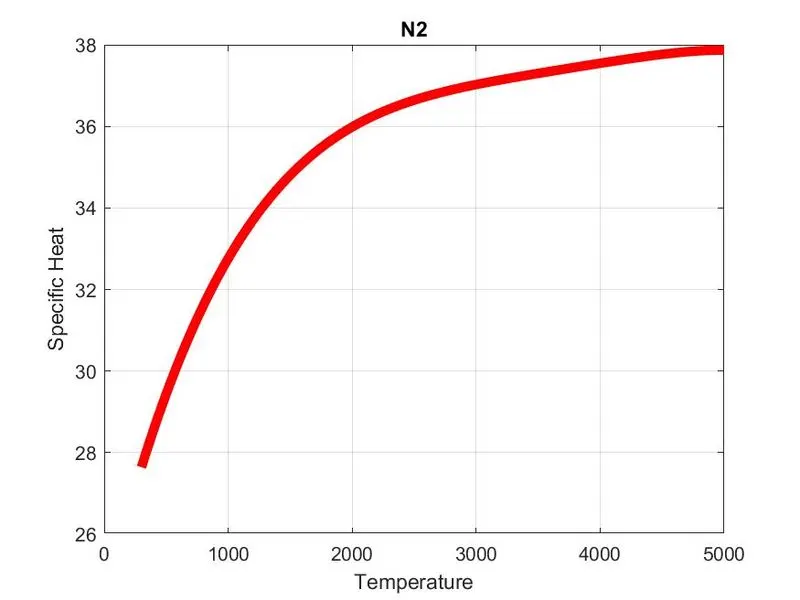
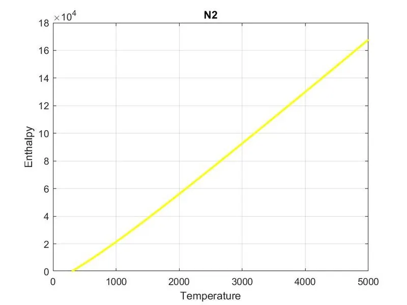
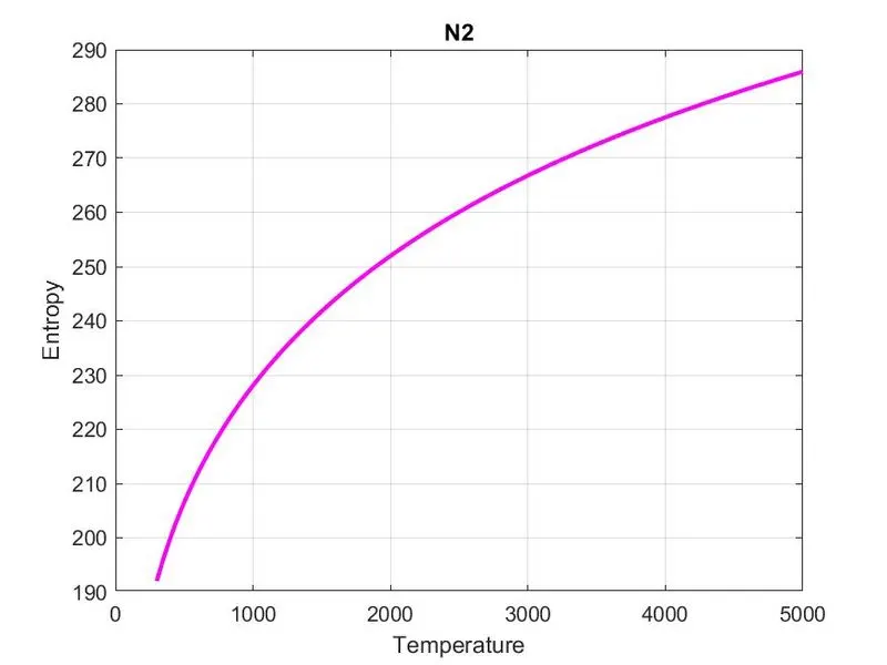
GRAPH FOR CO2:-

RESULT IN COMMAND WINDOWS:-

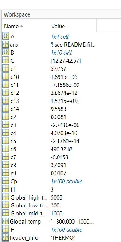
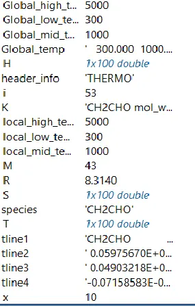
WORKSPACE RESULT:-

SCREENSHOT OF WINDOWS WHERE ALL THE PLOTS ARE SAVED: