Week 4.1 - Genetic Algorithm

AIM:- To write a code in Matlab to optimize the Stalagmite function and find Global Maxima of the function.

Theory:- Genetic Algorithm is a search -based optimisation technique.GA is based upon Evaluation theory propossed by Charle's Darvin and matlab has built in function for GA.The genetic algorithm repeatedly modifies a population of individual solutions.At each step,the GA select individuals at random from the current populationto be parents and uses them to produce the children for the next generation.

The genetic algorithm uses three main types of rules at each step to create the next generatiom from current population;

• Selection rules select the individuals, calles parents,that contribute to the populationat next generation.
• Crossover rules combine two parents to form children for next generation.
• Mutation rules apply random changes to individuals parents to form children.

Optimization:- Optimization is basically an area of study which deals with how to minimize or maximize the particular function which depends on multiple input parameters.

What is Stalagmites & Stalactites

Stalagmite is just amathematical model which helps us to generate local minimas & maximas. It is a type of a rock formaton that rises from the floor of a cave due to the accumulation of material deposited on the floor from ceiling drippings.

Stalactites are centimeter to meter hang from the ceiling & grow towards the cave floor.

Stalagmite Function:-

`f(x,y) = f1,xf2,xf1,yf2,y`

Where,

`f1,x =[sin(5.1pix+0.5)]^6`

`f1,y = [sin(5.1piy+0.5)]^6`

`f2,x = exp[-4ln(2)frac{(x-0.0667)^2}{0.64}]`

`f2,y=exp[-4ln(2)frac{(y-0.0667)^2}{0.64}]`

Syntax for genetic algorithm

We can give rhe inputs by following ways:

x = ga (fun,nvars)

x = ga(fun,nvars,A,b)

x = ga(fun,nvars,A,b,Aeq,beq)

x = ga(fun,nvars,A,b,Aeq,beq,lb,ub,nonlcon)

x = ga(fun,nvars,A,b,Aeq,beq,lb,ub,nonlcon,options)

x = ga(fun,nvars,A,b,[],[],lb,ub,nonlcon,Intcon)

x = ga(fun,nvars,A,b,[],[],lb,ub,nonlcon,IntCon,options)

x = ga(problem)

[x,fval] = ga(__)

[x,fval,exitflag,output] = ga(__)

[x,fval,exitflag,output,population,scores] = ga(__)

Syntax:

x = ga(fun,nvars)

x = ga(fun,nvars) finds a local unconstrained minimum, x, to the objective function,fun. nvars is the number of design variables of function,fun.

Outputs:-

[x,fval] = ga(__), for any previous input arguments,also returns fval,the value of the fitness function at x.

Code Explanation:-

1) x & y is the input arrays & this does not defined the search space for GA.It doesn't know that value can go beyond 0.6.

2)Since we need to plot a 3D surface plot we take the 2d array of x & y using meshgrid command & store them in input_vector array.

2)num_cases = 50 - running G.A. 50 times.

3)A nested loop was used to assign values from this array into an array named input_vector. input_vector is the input to the stalagmite function.

4)The stalagmite function is written seperately to reduce the complexity.

5)Minus (-) sign is given to the output of stalagmite functionso that, after the ga process it will get Global Maxima.

6)In the first case the bounds were not defined & the plots were made.Negative sign is given for f value inside surface function to get the stalgmite function upwords.

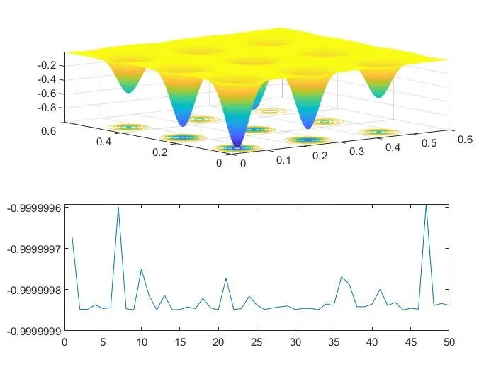
7)Bounding is given in next case so that the number of solutions approaches more accuracy.The population is increased in the subsequent cases & plotting is done.The Globa maxima is found in last case.

We can also used tic & toc command.

TOC:- The TOC function uses the recorded value to calculate elapsed time.

TIC:-Tic works with the TOC function to measure elapsed time.

The tic function records the current time.

Main Program

close all
clc

% Defining our search space
x = linspace(0,0.6,150);
y = linspace(0,0.6,150);
num_case = 50;

% Creating a two dimentional mesh
[xx, yy] = meshgrid(x,y);

% Evaluating the stalagmite function
for i = 1:length(xx)
    for j = 1:length(yy)
        input_vector(1)=xx(i,j);
        input_vector(2)=yy(i,j);
        f(i,j) = stalagmite(input_vector);
    end
end

%Study 1_unbounded 
tic
for i= 1:num_case
[input, fval(i)] = ga(@stalagmite,2) 
x_1(i)=input(1);
y_1(i)=input(2);

end
study_1 = toc

study_2 = tic 

    
figure(1)
subplot(2,1,1)
surfc(xx,yy,f);
shading interp
hold on
plot3(x_1,y_1,fval,'o-')
subplot(2,1,2)
plot(fval)


for i= 1:num_case
[input, fval_2(i)] = ga(@stalagmite,2,[],[],[],[],[0,0],[0.6,0.6]) 
x_1(i)=input(1);
y_1(i)=input(2);

end

study_2 = toc 

    
figure(2)
subplot(2,1,1)
surfc(xx,yy,f);
shading interp
hold on
plot3(x_1,y_1,fval_2,'o-')
subplot(2,1,2)
plot(fval_2)

%study_3
options=optimoptions('ga')
options=optimoptions(options,'populationsize',150);


for i= 1:num_case
[input, fval_2(i)] = ga(@stalagmite,2,[],[],[],[],[0,0],[0.6,0.6],[],[],options) 
x_1(i)=input(1);
y_1(i)=input(2);

end

study_3 = toc 

    
figure(3)
subplot(2,1,1)
surfc(xx,yy,f);
shading interp
hold on
plot3(x_1,y_1,fval_2,'o-')
subplot(2,1,2)
plot(fval_2)

Stalagmite Function Code:-

function F = stalagmite(input_vector)

x=input_vector(1);
y=input_vector(2);
f1=(sin((5.1*pi*x)+0.5))^6;
f2=(sin((5.1*pi*y)+0.5))^6;
f3=exp((-4*log(2)*((x-0.0667))^2/0.64));
f4=exp((-4*log(2)*((y-0.0667))^2/0.64));
F=(f1*f2*f3*f4*-1);

end

RESULTS:- FIGURE (1)

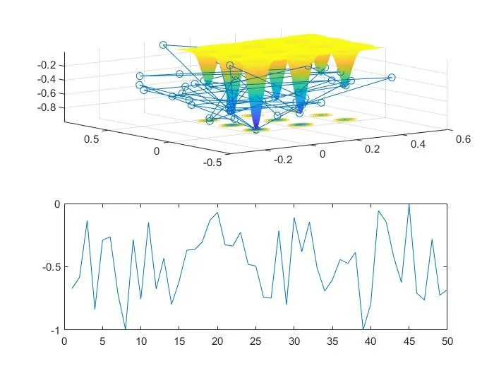
Here we can see the optimal values went outside the value of x.

So, we failes to reached the global maxima in this case.

The study time is 1.4983s

FIGURE (2)

Now lets focus on result of bounded values

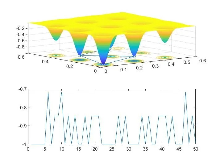
Throgh the optimum values are within the limits it could not give us the exact maxima values.

The study time is 3.7789s which is more than above study.

FIGURE (3)

In this case we are sucessful to find out the correct maxima for STALAGMITE function.

so by inncreasing the the initial popuation size of GA we can increase the accuracy of algorithm.

The study time is 8.9930

Reference:-

https://in.mathworks.com/discovery/genetic-algorithm.html