Week 3 - Solving second order ODEs

AIM:- Simulation of Simple Pendulum

Objective:- 

1.  To write a program that solves the ODE which represents the equation of motion of a simple pendulum with damping.
2.  Write a program in Matlab that will simulate the pendulum motion.

Theory:- A simple pendulum consist of mass m suspended with string having length L, when displaced by making some angles performs oscillatory motion.

Governing Damping Equation:- 

             

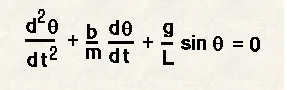
Where,

• b = damping coefficient;
• m = mass of bob in 'kg',
• g = gravity in 'm/s^2',                                                   
• l = length of pendulum in 'm'.

• b = 0.05
• m = 1 kg
• g = 9.81m/s^2
• l = 1m

Let's reduce the order of equation:- 

Let , `theta1` = `theta`

d`theta`/dt = d`theta1`/dt = `theta2`

Then the eqn. becomes:-

d^2`theta1`/dt + (b/m) d`theta1`/dt + (g/l)`sin``theta1`

also assume, d`theta1`/dt = `theta2`

So,

d`theta2`/dt + (b/m)(`theta2`) + (g/l)`sin``theta1`

From the above eqns we get ,

d`theta1`/dt  = `theta2`-----eqn(1)

d`theta2`/dt = -(b/m)`theta2` - (g/l)`sin``theta1`----eqn(2)

By combining we get Matrix:-

d/dt`````[[theta1],[theta2]]` =`[[theta2],[-(b/m)theta2 -(g/l)sin theta1]]`

By solving the matrix we get the values for `theta1`&`theta2` for the simple pendulum.

1) ode 45 Function is used in Matlab to solve ODE'S'

• MATLAB Code for the ode45 Function

function [dtheta_dt] = ode_func(t,theta,b,g,l,m)

theta1 = theta(1)
theta2 = theta(2)
dtheta1_dt = theta2;
dtheta2_dt = -(b/m)*theta2 - (g/1)*sin(theta1);
dtheta_dt = [dtheta1_dt; dtheta2_dt];

end

Matlab Code that will simulate the pendulum motion

clear all
close all
clc

b = 0.05;
g = 9.81;
l = 1;
m = 0.1;
ct = 1;

%initial condition
theta = [0;3];

%time points
t_span = linspace(0,20,500);

%solve ODE
[t,results] = ode45(@(t,theta)ode_func(t,theta,b,g,l,m),t_span,theta);

figure(1)
plot(t,results);
theta=results(:,1);
title('Time vs Displacement and Velocity');
xlabel('Time');
ylabel('Displacment and Velocity');
hold on


for c = 1:length(theta)
    Theta=theta(c);
 
x0 = 0
y0 = 0

x1 = l*sin(Theta);
y1 = -l*cos(Theta);

figure(2)
plot([-1 1],[0 0],'linewidth',6,'color','k');
title('Motion of Simple Pendulum');
hold on

plot([x0 x1],[y0 y1],'linewidth',3,'color','r');
hold on

plot(x1,y1,'o','markersize',25,'MarkerEdgeColor','r','MarkerFaceColor','g');
grid on
axis([-1 1 -1.5 1.5])
pause(0.03)

M(ct) = getframe(gcf);

hold off
ct=ct+1;

end

movie(M)
videofile = VideoWriter('pendulum_animation.avi','uncompressed AVI')
open(videofile)
writeVideo(videofile,M)
close(videofile)
        
        
        
    

FIGURE 1:-

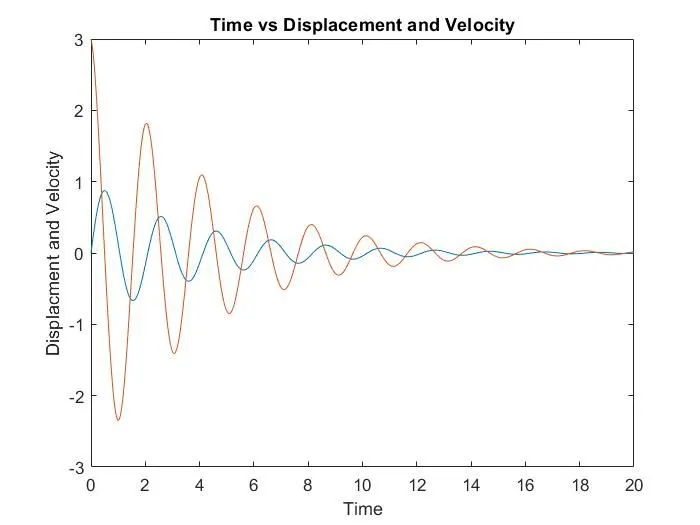
From the above graph, we can conclude that the displacement of pendulum is  decreasing with the progression of time due to effect of damping and same follwed by velocity, it also keeps on decreasing with respective time.

Animation of Motion of Simple pendulum :

The motion of simple pendulum is animated using for loop to capture each and every motion between given time interval.

Following link is provided to watch the animation of pendulum:-

https://drive.google.com/file/d/1z14B9LPO9_JuO51bKBuyMlCPYwxvFAgY/view?usp=sharing

Command used in above program :-

• 'o' is used to create sphere which is Marker code in Matlab.
• MarkerFacecolor, MarkerEdgecolor, Markersize to create sphere size, edge & face colour accordinglly.
• Movie command is used to create a movie