Project 2 - Rankine cycle Simulator

AIM:-

1. To create a Rankine cycle simulator using MATLAB.
2. Calculating all the states points of the cycle baesd on User inputs.
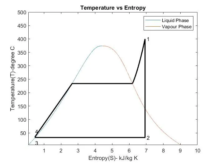
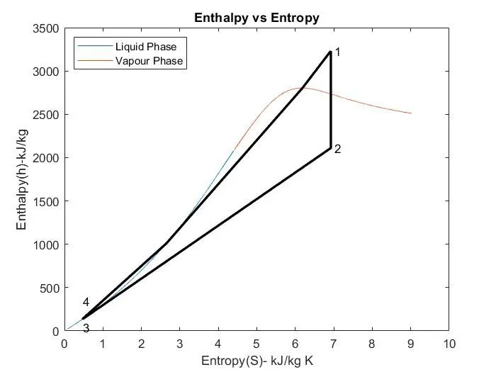
3. Plotting T vs S & H vs S plot for the given input.

RANKINE CYCLE

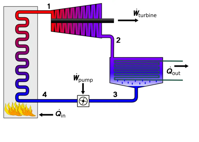
Rankine cycle is the process used in power plants. In this mechanism, a fuel is used to produce heat within a boiler,converting water into steam which then expands through a turbine producing useful work.This process was developed in 1859 by scottish engineer William J.M. Rankine.This is a thremodynamic cycle which converts heat into mechanical energy.

Procesess & Working of Rankine Cycle:-

There are four processes in the Rankine cycle:-

1. Process 1-2: Isentropic Expznsion in the turbine.
2. Process 2-3: Constant pressure Heat rejection in condenser
3. Process 3-4: Isentropic compression in the pump
4. Process 4-1: Constant pressure heat addition in the boiler

• Working of Rankine Cycle Simulator:-

1. In process 1-2, The dry saturated vapour expands through a turbine, generating power.This decreases the tmeperature & pressure of the vapour & some condensation may occcur.
2. In process 2-3, The vapour -liquid mixture leaving the turbine is condensed at low pressure, usually in a surface condensor using cooling water. In well designed & maintained condensor, the pressure of the vapour is below atmospheric pressure,approaching the saturation presure of the operating fluid at the cooling water temperature.
3. Process 3-4,The pressure of the condensate is raised in feed pump, Because of low specific volume of liquid,the ppump work is relatively small and often neglected in thermodynamic calculations.
4. Processs 4-1, High pressure liquid enters the boiler from feed pumpand is heated to the saturation temperature(on the saturation curve).Further addition of energy causes evaporation of the liquid untill it is fullly converted to saturated sream or superheated

Due to condensation step,the pressure at the turbine outlet is lowered.This means the pump requires less work to compress the water resulting in higher overall efficiencies.

Formula used:-

`W_net = Wt-Wp`

`Bwratio= frac{Wp}{Wt}`

`Wt = h1 -h2`

`Wp=h4-h3`

h is enthalpy at that state(kJ/Kg)

W_t is Turbine Work (Kj/Kg)

W_p is Pump Work(Kj/Kg)

Thermal Efficiency `(etat)`:-

`(etat)`= W_net/(Q_in)

Q_in = h1-h4;

where,

Q_in is Enthalpy at that state(Kj/Kg)

MAIN PROGRAM:-

clear all
close all
clc

disp('Rankine Cycle Simulator')
disp('process 1-2: Isentropic expansion in turbine ')
disp('process 2-3: constant pressure heat rejection in condenser')
disp('process 3-4: Isentropic Compression in pump')
disp('process 4-1: constant pressure heat addition in boiler')

% Intial data inputs
T1 = input('Enter the turbine inlet temp: ');
p1 = input('Enter the turbine inlet press: ');
p2 = input('Enter the turbine outlet press: ');


% State Point 1 parameters i.e Turbine Inlet
Tsat = XSteam('Tsat_p',p1);
h1 = XSteam('h_pt',p1,T1);
s1 = XSteam('s_pt',p1,T1);

%State Point 2 parameters i.e Condenser Inlet
s2 = s1;
sf2 = XSteam('sL_p',p2);
sg2 = XSteam('sv_p',p2);

% s2=sf2+(x2*sfg2)
% Dryness fraction
x2 =(s2-sf2)/(sg2-sf2);  

T2 = XSteam('T_ps',p2,s2);
h2 = XSteam('h_px',p2,x2);
hf2 = XSteam('hL_p',p2);

% State Point 3 Parameters i.e Pump Inlet
p3 = p2;
T3 = T2;
s3 = sf2;
h3 = hf2;
T5 = Tsat;

% State Point 4 Parameters i.e Boiler Inlet
s4 = s3;
p4 = p1;
h4=XSteam('h_ps',p4,s4);
cp=XSteam('cp_ps',p4,s4);
cv=XSteam('cv_ps',p4,s4);
c=cp/cv;
T4=T3*((p4/p3)^(c-1)/c)

% State Point 5,6 Parameters
T5=Tsat;
h5=XSteam('hL_p',p1);
s5=XSteam('sL_p',p1);
T6=T1;
h6=XSteam('hV_p',p1);
s6=XSteam('sV_p',p1);

% Plotting T-S Diagram
t=linspace(5,400,25000);
for i=1:length(t)
s(i)=XSteam('sL_t',t(i));
S(i)=XSteam('SV_t',t(i));
h(i)=XSteam('hL_t',t(i));
H(i)=XSteam('hV_t',t(i));
end
figure(1)
plot(s,t);
hold on
plot(S,t);

plot([s1,s2,s3,s4,s5,s6],[T1,T2,T3,T4,T5,Tsat],'linewidth',2,'color','k');
text(s1+0.1, T1, '1')
text(s2+0.1, T2, '2')
text(s3, T3-20, '3')
text(s4, T4+20, '4')
axis([1,10,10,500]);


% Plotting Saturated Temperature 
a=linspace(Tsat,T1,500);
for i=1:length(a)
    d(i)=XSteam('s_pt',p1,a(i));
end
plot(d,a,'linewidth',2,'color','k')
title('Temperature vs Entropy')
xlabel('Entropy(S)- kJ/kg K')
ylabel('Temperature(T)-degree C')
legend('Liquid Phase','Vapour Phase')


figure(2)
plot(s,h);
hold on
plot(S,H);

plot([s1,s2,s3,s4,s5,s6,s1],[h1,h2,h3,h4,h5,h6,h1],'linewidth',2,'color','k');
text(s1+0.1, h1, '1')
text(s2+0.1, h2, '2')
text(s3, h3-100, '3')
text(s4, h4 +200, '4')
title('Enthalpy vs Entropy')
xlabel('Entropy(S)- kJ/kg K')
ylabel('Enthalpy(h)-kJ/kg')
legend('Liquid Phase','Vapour Phase','location','northwest')

% Result to be displayed in the command window 
disp(' The following are the results of rankine cycle operation ')
disp(' ')
disp(' At the state point 1')
disp(' ')
n1=sprintf('p1 is %.2f bar',p1);
disp(n1)
n2=sprintf('T1 is %.2f Deg Celcius',T1);
disp(n2)
n3=sprintf('h1 is %.2f kJ/kg',h1);
disp(n3)
n4=sprintf('s1 is %.2f kJ/kgK',s1);
disp(n4) 

disp(' ')
disp(' At the state point 2')
disp(' ')
n5=sprintf('p2 is %.2f bar',p2);
disp(n5)
n6=sprintf('T2 is %.2f Deg Celcius',T2);
disp(n6)
n7=sprintf('h2 is %.2f kJ/kg',h2);
disp(n7)
n8=sprintf('s2 is %.2f kJ/kgK',s2);
disp(n8) 

disp(' ')
disp(' At the state point 3')
disp(' ')
n9=sprintf('p3 is %.2f bar',p3);
disp(n9)
n10=sprintf('T3 is %.2f Deg Celcius',T3);
disp(n10)
n11=sprintf('h3 is %.2f kJ/kg',h3);
disp(n11)
n12=sprintf('s3 is %.2f kJ/kgK',s3);
disp(n12) 

disp(' ')
disp(' At the state point 4')
disp(' ')
n13=sprintf('p4 is %.2f bar',p4);
disp(n13)
n14=sprintf('T4 is %.2f Deg Celcius',T4);
disp(n14)
n15=sprintf('h4 is %.2f kJ/kg',h4);
disp(n15)
n16=sprintf('s4 is %.2f kJ/kgK',s4);
disp(n16)

% Workdone by turbine

W_D_T = h1-h2

% Workdone by the pump

W_D_Pump = h4-h3

%net workdone

W_D_Net = W_D_T-W_D_Pump

% Heat Supplied
q = h1-h4;

% Effeciency
n = W_D_Net/q

% Specific steam consumption
ssc = 3600/W_D_Net

% Back Work Ratio
BWR = W_D_Pump/W_D_T

Expalination:-

• Xsteam data is used to extract steam and water properties of Enthalpy,entropy at specific pressure & temperautre for sat liquid,sat vapour conditions etc.
• The program requires the input of pressure at state pt 1(turbine inlet),Temperature at same point & Temp at condensor inlet
• with the help of inlets & Xsteam data, the program calculates all the state points of Rankine cycle.
• h = XSteam ('h_pT',p1,T1); returns the enthalpy of water at given pressure &temperature in bar & degC.
• As we extract data we used thermodynamic relations to find further state points.
• net work done,work done by turbine,work done to run the pump,heat in heat out are calculated using formulas.
• efficiency is also calculated.
• using plot commands plotted all state points.
• The plot changes as the user input changes for the above mentioned inputs.
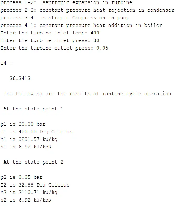
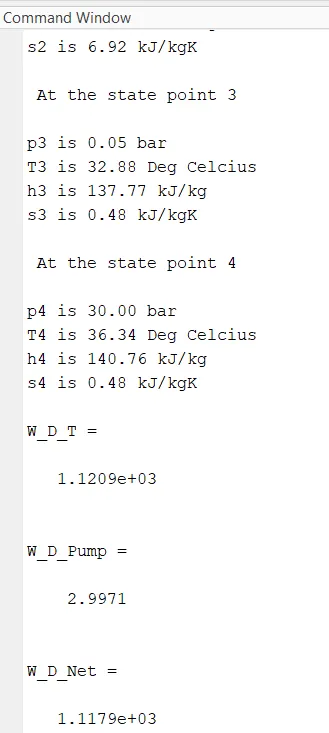
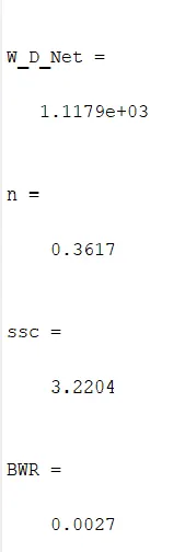
• Results are displayed in command windows.

RESULT IN COMMAND WINDOW:-

REFERENCE:-

https://energyeducation.ca/encyclopedia/Rankine_cycle