Challenge

Week 5 - Curve fitting

VVamsikrishna Bathala3 Jul 2021

1.what does popt and pcov mean?

popt:

it is an array of optimal values of parameters which minimizes the sum of squares of residuals.it is also known as an array of cofficient of polynomial for the sum squares of residual for given data is minimum in least square method

pcov:

2d array which contains the estimated covarience of popt . the diagnols provide the varience of popt.the diagnols provide the vaience of parameter estimate

2.what does np.array(temperature) do?

it is a command which provide access to the list of temperatures which are available in the data with the use of numpy command

3.what does the* in *popt mean?

it directs the compliers referance to all the values stored in the popt 1d array

* means all

4. write a code to fit linear and cubic polynomial for the Cp data.explian if results are good or bad

"""

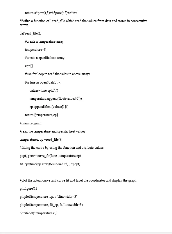
#program to curve fit the linear and cubic polynomials

"""

#imports modules such as numpy ,matplot and scipy to access the functions

import matplotlib.pyplot as plt

import numpy as np

from scipy.optimize import curve_fit

#define a function that represents the linear polynomial

def func(t,a,b,c):

return a*pow(t,2)+b*t+c

#define another function that represents the cubic polynomial

def cubic(t,a,b,c,d):

return a*pow(t,3)+b*pow(t,2)+c*t+d

#define a function call read_file which read the values from data and stores in consecutive arrays

def read_file():

#create a temperature array

temperature=[]

#create a specific heat array

cp=[]

#use for loop to read the vales to above arrays

for line in open('data','r'):

values= line.split(',')

temperature.append(float(values[0]))

cp.append(float(values[1]))

return [temperature,cp]

#main program

#read the temperature and specific heat values

temperature, cp =read_file()

#fitting the curve by using the function and attribute values

popt, pcov=curve_fit(func ,temperature,cp)

fit_cp=func(np.array(temperature) , *popt)

#plot the actual curve and curve fit and label the coordinates and display the graph

plt.figure(1)

plt.plot(temperature ,cp, 'r.',linewidth=3)

plt.plot(temperature, fit_cp, 'b.',linewidth=3)

plt.xlabel("temperatures")

plt.ylabel("Cp")

plt.legend(['actual_data','curve_fit'])

plt.show()

#read the temperature and specific heat values

temperature, cp =read_file()

#fitting the curve by using the function and attribute values

popt, pcov=curve_fit(cubic ,temperature,cp)

fit_cp=cubic(np.array(temperature) , *popt)

#plot the actual curve and curve fit and label the coordinates and display the graph

plt.figure(2)

plt.plot(temperature ,cp, 'r.',linewidth=3)

plt.plot(temperature, fit_cp, 'b.',linewidth=3)

plt.xlabel("temperatures")

plt.ylabel("Cp")

plt.legend(['actual_data','curve_fit'])

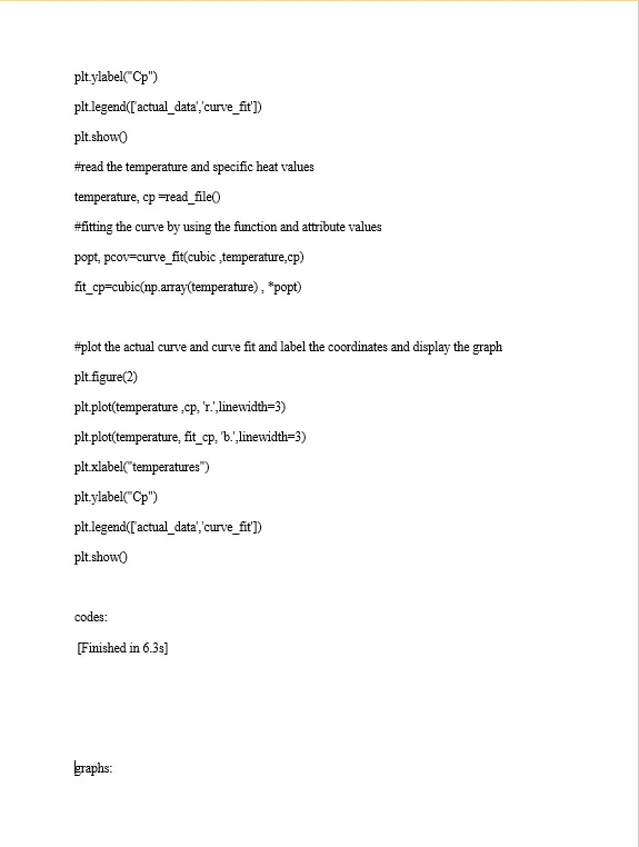
plt.show()

codes:

[Finished in 6.3s]

graphs:

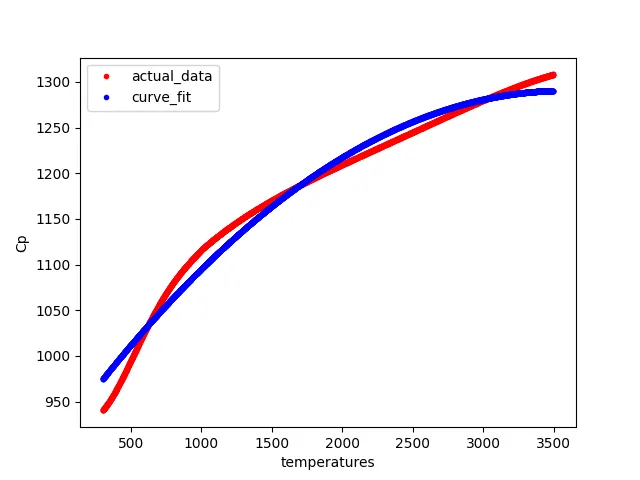
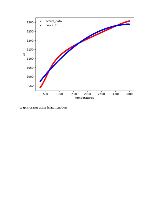
graphs drawn using linear function

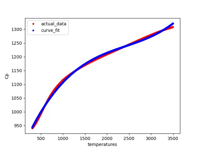
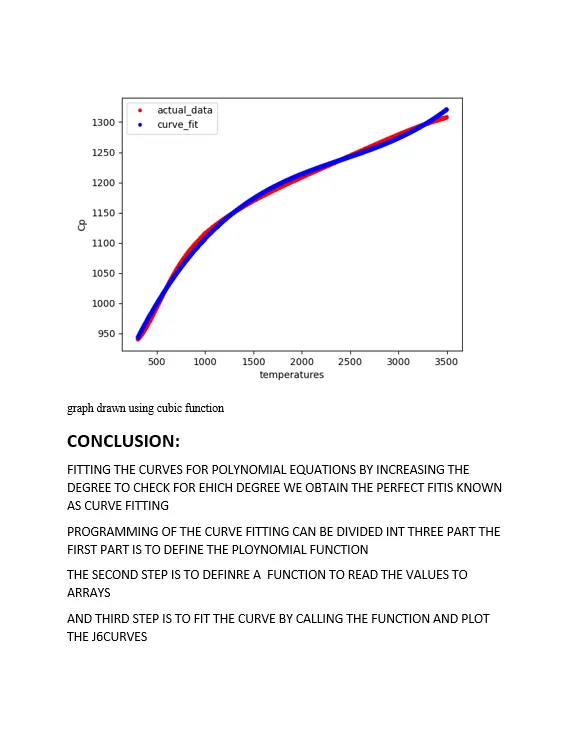
graph drawn using cubic function

5.what need to be done in order to make curve fit perfect?

by increasing the degree of polynomial we make make curtve fit perfect. fourth degree polynomial is considered as perfect curvefit when compared to the of a cubic polynomial.increasing the degree makes the calculations complicated such that fourth degree polynomial is considered as perfect curve fit

6.show empirically how well the curve has been fit

from the above two graphs cubic polynomial has fit the curve more accurately when compared to that of the linear equation

by results we can say that increasing the degree of the polynomial makes the accurate fit

Report: