Week 2 Air standard Cycle
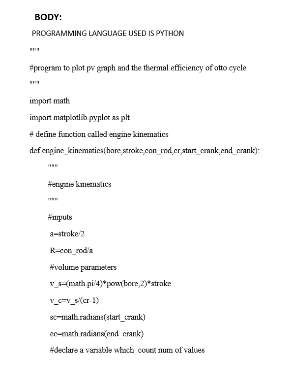
"""
#program to plot pv graph and the thermal efficiency of otto cycle
"""
import math
import matplotlib.pyplot as plt
# define function called engine kinematics
def engine_kinematics(bore,stroke,con_rod,cr,start_crank,end_crank):
"""
#engine kinematics
"""
#inputs
a=stroke/2
R=con_rod/a
#volume parameters
v_s=(math.pi/4)*pow(bore,2)*stroke
v_c=v_s/(cr-1)
sc=math.radians(start_crank)
ec=math.radians(end_crank)
#declare a variable which count num of values
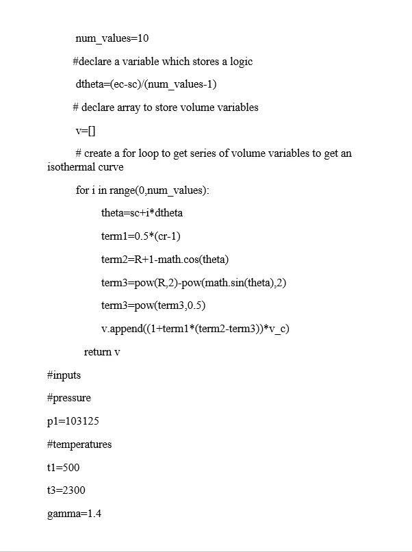
num_values=10
#declare a variable which stores a logic
dtheta=(ec-sc)/(num_values-1)
# declare array to store volume variables
v=[]
# create a for loop to get series of volume variables to get an isothermal curve
for i in range(0,num_values):
theta=sc+i*dtheta
term1=0.5*(cr-1)
term2=R+1-math.cos(theta)
term3=pow(R,2)-pow(math.sin(theta),2)
term3=pow(term3,0.5)
v.append((1+term1*(term2-term3))*v_c)
return v
#inputs
#pressure
p1=103125
#temperatures
t1=500
t3=2300
gamma=1.4
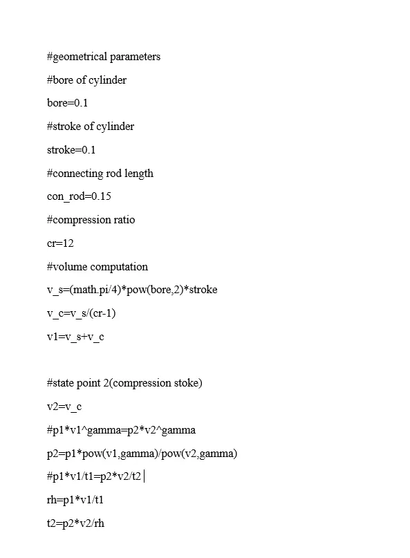
#geometrical parameters
#bore of cylinder
bore=0.1
#stroke of cylinder
stroke=0.1
#connecting rod length
con_rod=0.15
#compression ratio
cr=12
#volume computation
v_s=(math.pi/4)*pow(bore,2)*stroke
v_c=v_s/(cr-1)
v1=v_s+v_c
#state point 2(compression stoke)
v2=v_c
#p1*v1^gamma=p2*v2^gamma
p2=p1*pow(v1,gamma)/pow(v2,gamma)
#p1*v1/t1=p2*v2/t2
rh=p1*v1/t1
t2=p2*v2/rh
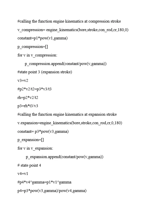
#calling the function engine kinematics at compression stroke
v_compression= engine_kinematics(bore,stroke,con_rod,cr,180,0)
constant=p1*pow(v1,gamma)
p_compression=[]
for v in v_compression:
p_compression.append(constant/pow(v,gamma))
#state point 3 (expansion stroke)
v3=v2
#p2*v2/t2=p3*v3/t3
rh=p2*v2/t2
p3=rh*t3/v3
#calling the function engine kinematics at expansion stroke
v.expansion=engine_kinematics(bore,stroke,con_rod,cr,0,180)
constant= p3*pow(v3,gamma)
p_expansion=[]
for v in v_expansion:
p_expansion.append(constant/pow(v,gamma))
# state point 4
v4=v1
#p4*v4^gamma=p1*v1^gamma
p4=p3*pow(v3,gamma)/pow(v4,gamma)
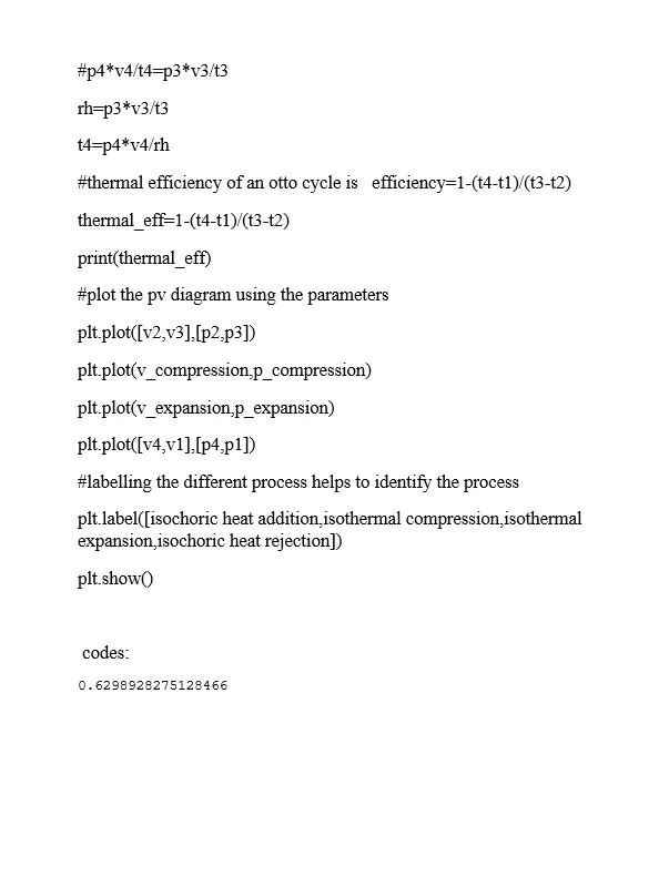
#p4*v4/t4=p3*v3/t3
rh=p3*v3/t3
t4=p4*v4/rh
#thermal efficiency of an otto cycle is efficiency=1-(t4-t1)/(t3-t2)
thermal_eff=1-(t4-t1)/(t3-t2)
print(thermal_eff)
#plot the pv diagram using the parameters
plt.plot([v2,v3],[p2,p3])
plt.plot(v_compression,p_compression)
plt.plot(v_expansion,p_expansion)
plt.plot([v4,v1],[p4,p1])
#labelling the different process helps to identify the process
plt.label([isochoric heat addition,isothermal compression,isothermal expansion,isochoric heat rejection])
plt.show()
codes:
0.6298928275128466
[Finished in 25.0s]
p-v diagram:
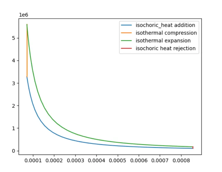
REPORT:
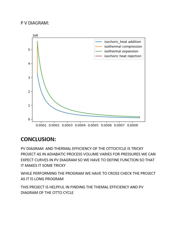
PV DIAGRAM OF AN OTTO CYCLE: