Week 3 - Solving second order ODEs
"""
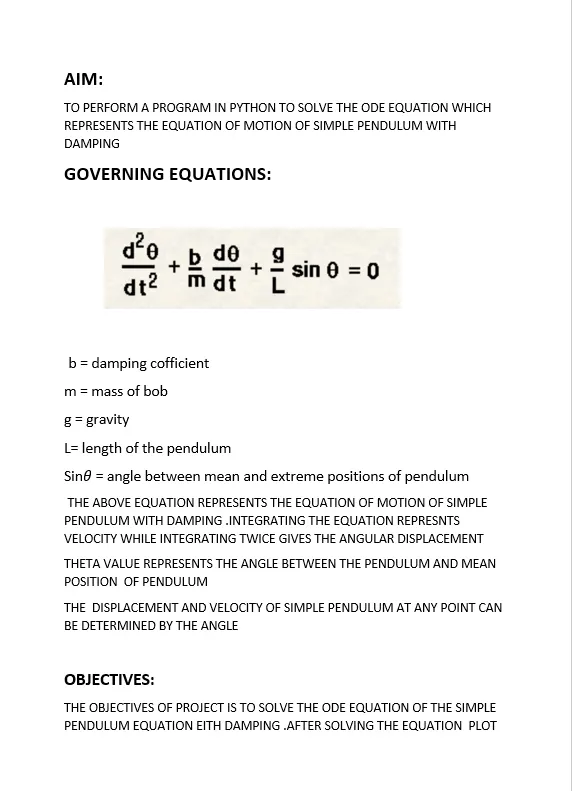
#program to solve ODE equation represents the equation of motion with simple pendulum with damping
"""
#import modules such as numpy to use matrix functions,math for mathamatical functions ,scipy to solve to integrate differenctial equations and matplot to plotting the graphs
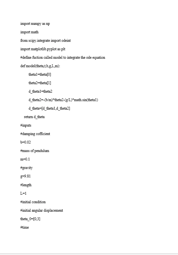
import numpy as np
import math
from scipy.integrate import odeint
import matplotlib.pyplot as plt
#define fuction called model to integrate the ode equation
def model(theta,t,b,g,L,m):
theta1=theta[0]
theta2=theta[1]
d_theta1=theta2
d_theta2=-(b/m)*theta2-(g/L)*math.sin(theta1)
d_theta=[d_theta1,d_theta2]
return d_theta
#inputs
#damping cofficient
b=0.02
#mass of pendulum
m=0.1
#gravity
g=9.81
#length
L=1
#initial condition
#initial angular displacement
theta_0=[0,3]
#time
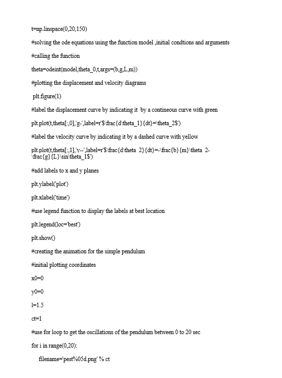
t=np.linspace(0,20,150)
#solving the ode equations using the function model ,initial condtions and arguments
#calling the function
theta=odeint(model,theta_0,t,args=(b,g,L,m))
#plotting the displacement and velocity diagrams
plt.figure(1)
#label the displacement curve by indicating it by a contineous curve with green
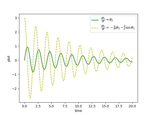
plt.plot(t,theta[:,0],'g-',label=r'$\frac{d\theta_1}{dt}=\theta_2$')
#label the velocity curve by indicating it by a dashed curve with yellow
plt.plot(t,theta[:,1],'y--',label=r'$\frac{d\theta_2}{dt}=-\frac{b}{m}\theta_2-\frac{g}{L}\sin\theta_1$')
#add labels to x and y planes
plt.ylabel('plot')
plt.xlabel('time')
#use legend function to display the labels at best location
plt.legend(loc='best')
plt.show()
#creating the animation for the simple pendulum
#initial plotting coordinates
x0=0
y0=0
l=1.5
ct=1
#use for loop to get the oscillations of the pendulum between 0 to 20 sec
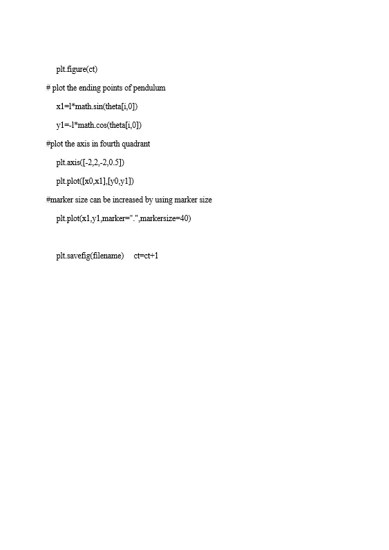
for i in range(0,20):
filename='pest%05d.png' % ct
plt.figure(ct)
# plot the ending points of pendulum
x1=l*math.sin(theta[i,0])
y1=-l*math.cos(theta[i,0])
#plot the axis in fourth quadrant
plt.axis([-2,2,-2,0.5])
plt.plot([x0,x1],[y0,y1])
#marker size can be increased by using marker size
plt.plot(x1,y1,marker=".",markersize=40)
plt.savefig(filename)
ct=ct+1
codes:
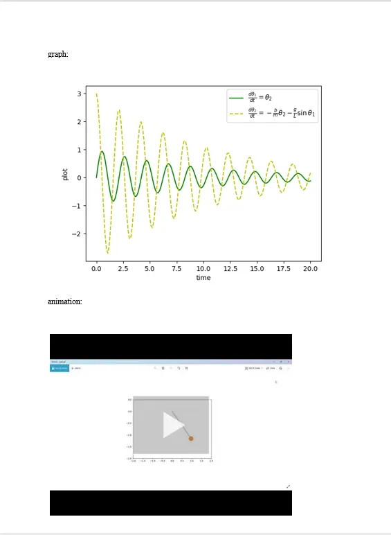
[Finished in 32.4s]graph:
animation:
REPORT:
ANIMATION: